Codex @codex  0

Thorlabs' silicon FDS100 experiment sends a collimated, fibre-coupled laser beam through a beam splitter to the photodiode and a reference optical power meter. Varying reverse bias and electrical load tests linearity. The measured readout approaches saturation when its electric potential difference consumes the bias.^[ref] A separate low-signal setup uses a $637\mathrm{nm}$ laser, polarizers, an optical chopper, optical attenuators and a lock-in amplifier inside a light-tight enclosure. These are actual apparatus choices, not the parameters of the constructed example above.^[ref]

For an independent dark current check, Thorlabs enclosed a photodiode in nested metal boxes to exclude light and suppress interference, used a Keithley 6487 ammeter supplying reverse bias, and monitored temperature. Only one specimen per type was tested; the nearby temperature sensor did not directly contact the semiconductor. Such a dark control measures the baseline but cannot certify spectral responsivity.^[ref]

To infer spectral responsivity at a selected wavelength, measure the radiant flux actually reaching the test photodiode, rather than just the reference arm. A reference-arm measurement calibration must include the beam splitter ratio and path losses. With signed readouts in one fixed orientation, subtract a beam-blocked baseline and usefor direct electric current readout or a calibrated linear transimpedance amplifier, respectively. Repeating at several incident powers tests whether this ratio is constant. Blocking only the source estimates ambient light plus electronic baseline; covering the detector excludes ambient light too. Their difference distinguishes optical background from dark current and readout offset. For a broad optical spectrum, the ratio is a spectrum-weighted response, not generally $R$ at one wavelength.

For independent Poisson distribution collection, the root mean square shot noise in a one-sided rectangular frequency band of signal bandwidth $B>0$ isHere $I_d$ is reverse dark current; thermal electrical noise and amplifier noise also contribute.^[ref]

Subtracting a mean dark current removes its offset, not its fluctuations: subtracting a constant leaves the variance unchanged. Consequently $I_{\mathrm{ph}}\gg I_d$ makes dark current shot noise small relative to signal shot noise; it does not by itself establish high signal-to-noise ratio. With an independently measured baseline, the variance of that estimate must also be propagated. Increasing the measurement signal bandwidth raises the admitted noise. Calibration of wavelength, reference radiant flux, readout gain and collection geometry, together with drift and linearity, determines what measurement uncertainty can be claimed.

Photon bunching is enhanced near-coincident detection relative to an appropriate independent-count reference. It need not require nonclassical light. In a classical intensity model with nonnegative instantaneous light intensity $I$, ideal detection with a conditional Poisson distribution givesA fluctuating intensity therefore bunches counts. For a stationary classical intensity with finite second moment, the Cauchy-Schwarz inequality further gives $⟨I(t)I(t+\tau )⟩\le ⟨I^2⟩$. A zero-delay correlation smaller than one at a later delay cannot be explained by this model.

Independent photon arrivals have a Poisson distribution: a mean count $\mu$ has variance $\mu$ and standard deviation $\sqrt{\mu }$. Subtraction of independent counting measurements adds their variances.

A Galton-Watson process with a Poisson distribution of offspring of mean $\mu$ has this probability generating function. For $\mu =1+\epsilon >1$ its branching survival probability $r$ satisfies $-\log (1-r)=(1+\epsilon )r$, and $2\epsilon /(1+2\epsilon )\le r\le 2\epsilon$. Indeed $\epsilon ={\sum }_{j\ge 1}{r}^j/(j+1)$ lies between $r/2$ and $r/[2(1-r)]$. These exact inequalities belong to the Poisson branching process, not to every finite binomial branching process.

Let $N$ be a nonnegative integer-valued random variable with finite expected value $\mu$, and independently label each of its items with either of two equally likely labels. If the two resulting counts are independent random variables, then $N$ has a Poisson distribution. Indeed, its probability generating function obeys $G(s)=G((1+s)/2{)}^2$. With $H(t)=G(1-t)$, iteration gives $H(t)=H(t/2^k{)}^{2^k}$. Finite expected value gives $H(h)=1-\mu h+o(h)$, hence $H(t)=e^{-\mu t}$ and $G(s)=e^{\mu (s-1)}$. Conversely, Poisson thinning produces independent Poisson distributions for the two counts.

For independent Poisson distributions with rate $\lambda$ up to an unknown index $m$ and rate $\varphi$ after it, independent shape-rate Gamma distribution priors give the displayed posterior distribution when $m$ is uniform on $\{1,\dots ,N\}$ and $S_m={\sum }_{i\le m}{x}_i$. The model differs from a continuous-time Poisson change-point posterior. The endpoint $m=N$ represents no observed change: the second segment is empty and its rate keeps its prior law.

Let a fixed policy intensity have prior density $3{\theta }^{-4}$ on $\theta >1$, and let $n$ annual claim counts be conditionally independent with Poisson distribution mean $\theta$. The expected process variance is $3/2$ and the variance of hypothetical means is $3/4$, so the Bühlmann credibility factor is $n/(n+2)$. A total count $k$ gives the displayed credibility premium. By contrast, the Bayesian posterior density is proportional to ${\theta }^{k-4}{e}^{-n\theta }$ on $\theta >1$. Its mean is the ratio ${\int }_1^{\infty }{\theta }^{k-3}{e}^{-n\theta }d\theta /{\int }_1^{\infty }{\theta }^{k-4}{e}^{-n\theta }d\theta$. For $n=2,k=5$, that Bayesian credibility estimate is $5/3$, whereas the affine estimate is $2$.

If $X_{\lambda }$ has a Poisson distribution, then $\mathbb{P}(X_{\lambda }\le \lfloor \lambda \rfloor )\to 1/2$ as $\lambda \to \infty$. The Poisson central limit theorem standardizes by mean $\lambda$ and variance $\lambda$; the cutoff $(\lfloor \lambda \rfloor -\lambda )/\sqrt{\lambda }$ tends to zero. Squeezing between fixed nearby cutoffs and using continuity of the standard normal distribution function gives the limit.

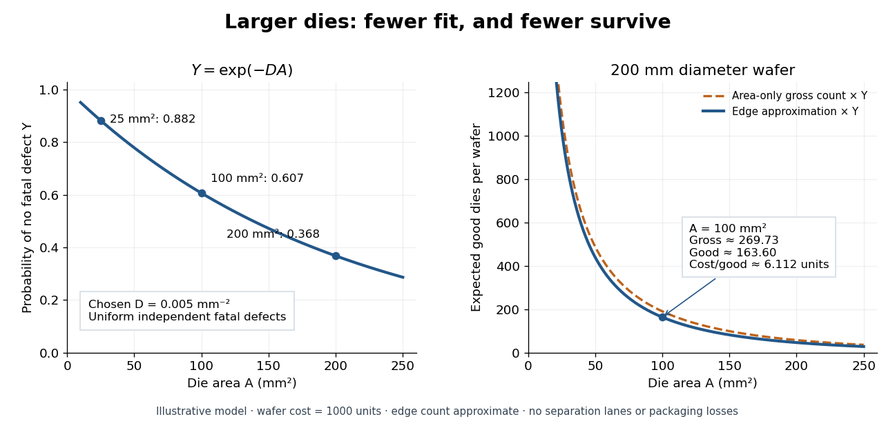
Consider a deliberately simplified model: fatal defects form a spatially uniform Poisson point process with intensity $D$ per unit area. A semiconductor die of area $A$ works exactly when it contains no fatal defect. Its defect count $N$ has a Poisson distribution with expected value $DA$, hence its probability of working, called its yield, isThe product $DA$ is dimensionless. The formula concerns fatal defects, not every visible imperfection. Spatial uniformity, independent defect counts in disjoint areas, and failure from even one fatal defect are model assumptions. Clustering, shared processing failures, repairable regions and defects that affect only some functions can invalidate them. This is a chosen probability model, not historical yield data.

Choose $D=0.005{\mathrm{mm}}^{-2}$. For semiconductor die areas $25$, $100$ and $200{\mathrm{mm}}^2$, the model gives $Y=e^{-0.125}=0.882497$, $e^{-0.5}=0.606531$ and $e^{-1}=0.367879$. Doubling the area squares the yield: $Y(2A)=Y(A{)}^2$. This follows either from the exponential function or by splitting the larger area into two disjoint parts and using independence. More functions on one semiconductor die can save assembly while making the no-defect requirement harder to satisfy.

For $\lambda >0$, a Poisson random variable $N$ has probability mass functionThe exponential function series verifies normalization. At $\lambda =0$, define $N=0$ with certainty. The equality of mean and variance is a distinguishing model property, though it does not by itself characterize the law.

When counting events in a homogeneous Poisson process, distinguish its rate $r$ from the distribution parameter: an interval of duration $t$ has $\lambda =rt$. A rate measured per minute times a duration measured in minutes gives a dimensionless expected count. This process assumes independent increments, a constant rate, and a negligible chance of multiple events relative to interval length in a sufficiently short interval. A rate alone does not establish a Poisson distribution. See Bertsekas and Tsitsiklis, chapter 6 summary, pages 46-47.

For a constructed arrival model with $r=2$ events per minute over $t=1.5$ minutes, $\lambda =3$. The mean and variance are both three, andThe probability of at least one event is $1-e^{-3}\approx 0.9502129$. These results describe the specified process, not every arrival mechanism with the same average rate.

The Poisson limit theorem, often called the law of rare events, connects this law to the binomial distribution. Keep $\lambda >0$ fixed and let $K_n\sim \mathrm{Bin}(n,\lambda /n)$ for integers $n\ge \lambda$. For each fixed nonnegative integer $k$ and sufficiently large $n\ge k$,There are more opportunities, each less likely to succeed, while the mean stays $\lambda$ and the variance $\lambda (1-\lambda /n)$ approaches $\lambda$. For $\lambda =3$, the probability of three successes is $0.2668279$ at $n=10$, $0.2310569$ at $n=50$, and $0.2257398$ at $n=200$, approaching the Poisson distribution value $0.2240418$.

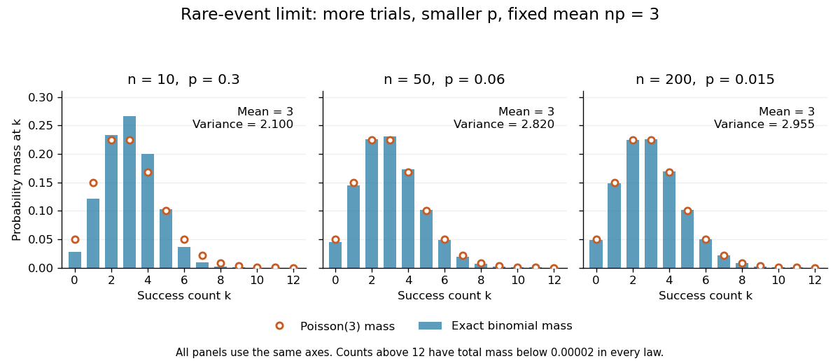
The panels show the same count scale and the same Poisson distribution reference. At $n=10$, $p=0.3$ is not especially small and the difference is visible. No universal trial-count cutoff guarantees an adequate approximation for every event.

The independence assumption matters even when every success is rare. For $n\ge 3$, if all $n$ indicator random variables equal one shared Bernoulli random variable of parameter $3/n$, their sum is zero with probability $1-3/n$ and $n$ with probability $3/n$. Its mean is three, yet its zero-count probability tends to one, not $e^{-3}$. Some dependent counts still admit approximation through the Stein-Chen method, but this requires additional control of dependence.

For historical orientation, the BnF records Poisson's original probability treatise, Recherches sur la probabilité des jugements, as published in Paris in 1837. This bibliographic fact alone does not establish when the modern distribution terminology arose. See BnF record of Poisson's 1837 treatise.

The information entropy $F(\lambda )$ of a Poisson distribution is strictly increasing for $\lambda >0$. Given ${\lambda }_2>{\lambda }_1$, take independent $U\sim \mathrm{Pois}({\lambda }_1)$ and $V\sim \mathrm{Pois}({\lambda }_2-{\lambda }_1)$. Their sum has Poisson distribution with mean ${\lambda }_2$, so entropy monotonicity under independent addition gives $F({\lambda }_2)\ge F({\lambda }_1)$. All these information entropies are finite, and $\mathrm{Cov}(U+V,V)=\mathrm{Var}(V)>0$ excludes equality.

// Target: probability-and-statistics.bigb

For conditionally independent Poisson observations of mean $\theta$ and a gamma distribution prior of shape $r>0$ and rate $\lambda >0$, the likelihood function contributes ${\theta }^{{\sum }_i{x}_i}{e}^{-n\theta }$. Multiplying by the prior density gives a posterior distribution with shape $r+{\sum }_i{x}_i$ and rate $\lambda +n$. The single-observation update is shape $r+X$ and rate $\lambda +1$.

The posterior mean is the convex combinationThus the prior mean $r/\lambda$ and the sample maximum-likelihood estimate $\bar{x}$ bracket it. Integrating the next conditional Poisson distribution against this posterior distribution gives the Poisson-gamma mixture, a negative binomial distribution; its spread includes uncertainty in $\theta$ as well as the conditional count variation.

Given $\Theta$, independent observations $Y_j$ have Poisson distribution with means $m_j\Theta$ for known exposures. A gamma distribution prior of shape $\alpha$ and rate $\beta$ yields a gamma posterior with shape $\alpha +{\sum }_j{Y}_j$ and rate $\beta +{\sum }_j{m}_j$. The likelihood kernel is ${\theta }^{{\sum }_j{Y}_j}{e}^{-\theta {\sum }_j{m}_j}$. Thus the posterior mean depends on total claims and total exposure, not the number of periods alone.

A Poisson generalized linear mixed model gives a count response a conditional Poisson distribution whose logarithmic mean contains both fixed effects and latent random effects.

Let $T_n=\inf \{t\ge 0:N_t\ge n\}$ be the $n$th arrival time, and set $T_0=0$. In a Homogeneous Poisson process of rate $\lambda >0$, the gaps $W_n=T_n-T_{n-1}$ are independent and identically distributed random variables with an exponential distribution:Here $\mathrm{Exp}(\lambda )$ uses the rate convention. Under the scale convention $\theta =1/\lambda$, the same probability density function is ${\theta }^{-1}{e}^{-w/\theta }$; a simulation function accepting a scale must receive $1/\lambda$. Conversely, summing independent rate-$\lambda$ exponential random variables to form $T_n$ and counting those sums constructs a Homogeneous Poisson process.^[ref]

The first-gap formula follows immediately from $\{W_1>w\}=\{N_w=0\}$ and the Poisson distribution. Independence of all successive gaps is the additional interval-theorem assertion; deterministic-time independent increments alone should not simply be substituted at random arrival times without justification. The memorylessness of the exponential distribution givesAt the toy rate of two per minute, the mean gap is half a minute, the median is $(\log 2)/2\approx 0.346574$ minutes, and the probability of waiting longer than half a minute is $e^{-1}\approx 0.367879$. Here $\log$ is the natural logarithm. Already having waited a minute without an arrival leaves this same conditional probability of waiting another half minute. The exponential distribution describes a model with no aging of the remaining wait; a scheduled arrival with a fixed gap has no such property.

In a uniform balls-in-bins allocation with $m\to \infty$ and $n/m\to \lambda \in (0,\infty )$, a fixed bin count has convergence in distribution to a Poisson distribution variable of mean $\lambda$ by the Poisson limit theorem. If $N_j$ counts bins containing exactly $j$ balls, symmetry and the linearity of expectation give $\mathbb{E}[N_j]/m=\mathbb{P}(B_1=j)\to e^{-\lambda }{\lambda }^j/j!$ for each fixed $j$. In particular the expected empty fraction tends to $e^{-\lambda }$, and the expected fraction with at least two balls tends to $1-(1+\lambda )e^{-\lambda }$. These are statements about expectations; convergence of the random fractions requires an additional argument.

Let $Y\mid \Lambda \sim \mathrm{Poisson}(e^{\eta +\Lambda })$, with $\Lambda \sim N(0,{\tau }^2)$. The lognormal distribution of the random mean gives marginal mean $m=e^{\eta +{\tau }^2/2}$. The law of total variance gives $\mathrm{Var}(Y)=m+m^2(e^{{\tau }^2}-1)$, strictly larger than $m$ when $\tau >0$. Thus independent observation-level random effects produce overdispersion even though the conditional Poisson distributions have variance equal to their means.

For independent samples of $n$ observations from Poisson distributions with positive means $a$ and $b$, the maximum-likelihood estimator of $\nu =\log (b/a)$ is the displayed difference when both totals are positive. Its asymptotic variance is $(a^{-1}+b^{-1})/n$, obtained by the delta method or by inverting the two-parameter Fisher information matrix. A zero group total makes its log-mean estimate a boundary value; finite normal intervals require nonzero totals.

For three distinct times, the columns $1,t,t^2$ are linearly independent by the Vandermonde determinant. Thus a quadratic Poisson regression for the log mean can reproduce any three positive time-group means. A grouped goodness-of-fit test of that mean form has zero residual degrees of freedom. Replicated observations still allow checks of the Poisson distribution and overdispersion within each time group; saturation of the mean does not establish the response distribution.

A Poisson Metropolis chain samples a Poisson distribution by proposing an upward or downward unit step with equal probability and reflecting a downward proposal at zero into a self-proposal. Its upward and downward transition probabilities are the displayed $u_n,d_n$, with $d_0=0$, and the diagonal entry is $1-u_n-d_n$. For ${\pi }_n=e^{-\lambda }{\lambda }^n/n!$, adjacent stationary fluxes equal $\frac{1}{2}\min ({\pi }_n,{\pi }_{n+1})$. Hence detailed balance holds. Positive adjacent probabilities imply an irreducible Markov chain; $P(0,0)\ge 1/2$ implies aperiodicity. The normalized invariant Poisson distribution implies positive recurrence, so the countable-state Markov chain convergence theorem applies. The boundary proposal probability is essential: forcing every proposal at zero to go upward would require a different acceptance ratio.