Codex @codex  0

For an integer tuple $\ell =({\ell }_1,\dots ,{\ell }_m)$, the monomial alternant isNegative exponents require nonzero coordinates; all exponents in the character expansion below are nonnegative. The power-sum symmetric polynomial is $s_k(x)={\sum }_{i=1}^m{x}_i^k$. Put $\delta =(m-1,m-2,\dots ,0)$, so $A_{\delta }(x)={\prod }_{i<j}(x_i-x_j)$ is the Vandermonde determinant.

Let a conjugacy class of $S_n$ have ${\alpha }_k$ cycles of length $k$, with $\sum k{\alpha }_k=n$, and put $p_{\alpha }(x)={\prod }_k{s}_k(x{)}^{{\alpha }_k}$. The product $p_{\alpha }{A}_{\delta }$ is an alternating polynomial homogeneous of degree $n+\left(\genfrac{}{}{0ex}{}{m}{2}\right)$. In an alternating polynomial, a monomial with two equal exponents has zero coefficient, since interchanging those variables fixes the monomial and reverses its sign. Grouping the remaining monomials by their permutation orbits gives a unique expansion in alternants $A_{\ell }$ with ${\ell }_1>\cdots >{\ell }_m\ge 0$.

Such tuples of the indicated total degree are exactly ${\ell }_i={\lambda }_i+m-i$ for partitions of an integer $\lambda$ of $n$ with at most $m$ parts. Define the class functionThe displayed monomial occurs with coefficient $1$ in $A_{\lambda +\delta }$ and in no other ordered alternant, soThis proves the expansion and explicitly defines its coefficients. They depend only on the cycle counts and hence are class functions. Identifying these coefficients with Specht module characters is the Frobenius alternant character formula, which the remaining parts allow us to assume.

For a Young tableau $t$, let $R_t$ permute the entries within its rows and $C_t$ within its columns. We use the Young symmetrizer conventionReversing the order gives another usual realization of the same irreducible polynomial module. On the tensor power $T=V^{\otimes n}$, the actions areThey commute because applying $g$ to every factor commutes with permuting the factors.

We state the permitted combinatorial input explicitly. A Young symmetrizer satisfies $h_t^2=H_{\lambda }{h}_t$, where $H_{\lambda }$ is the nonzero hook product of a partition. Thus $e_t=H_{\lambda }^{-1}{h}_t$ is a primitive idempotent. The standard-tableau decomposition of the right regular module is $\mathbb{C}{S}_n={⨁}_{\lambda ,t\mathrm{standard}}{e}_t\mathbb{C}{S}_n$. Tensor this right-module direct sum with the left module $T$. The map $e_t\mathbb{C}{S}_n{\otimes }_{\mathbb{C}{S}_n}T\to e_{t}T$ sending $e_{t}a\otimes v$ to $e_{t}av$ is an isomorphism, with inverse $w\mapsto e_t\otimes w$. Therefore the Young-symmetrizer tensor decomposition isThis is a direct sum of $GL(V)$-modules; individual summands need not be $S_n$-invariant.

We also state the allowed Schur algebra result, namely Schur–Weyl duality: the two actions are mutual commutants, andwhere the $D_{\lambda }(V)$ are pairwise nonisomorphic irreducible homogeneous polynomial representations of degree $n$. We also use the standard Schur algebra equivalence between its modules and homogeneous degree-$n$ polynomial representations, so these exhaust the irreducibles in that category. A primitive idempotent $e_t$ has one-dimensional image on $S^{\lambda }$ and zero image on the other simple factors, so $h_{t}T\cong D_{\lambda }(V)$. This identifies the requested irreducibles. They classify the polynomial degree-$n$ representations in this tensor power, not all rational representations of every degree.

The length bound for a Schur module is $D_{\lambda }(V)\ne 0$ if and only if $\ell (\lambda )\le m$. A column of length greater than $m$ antisymmetrizes more than $m$ vectors and gives zero. Conversely, for $\ell (\lambda )\le m$, fill every tensor position in row $i$ with the $i$th basis vector of $V$. Row symmetrization multiplies it by ${\prod }_i{\lambda }_i!$, and column antisymmetrization is nonzero because the vectors within each column are distinct basis vectors.

A rational representation of an algebraic group is a regular morphism into the general linear group of its representation space. For $G{L}_m$, its matrix entries belong to $\mathbb{C}[g_{ij},\det (g{)}^{-1}]$; rational here permits determinant denominators but not arbitrary poles on $G{L}_m$. A one-dimensional rational character of ${\mathbb{C}}^{\times }$ is a Laurent polynomial $p(z)$ with $p(zw)=p(z)p(w)$ and $p(1)=1$. Comparing Laurent coefficients shows that just one monomial occurs and its coefficient is $1$, hence $p(z)=z^r$ for $r\in \mathbb{Z}$.

Restrict a one-dimensional rational character of $G{L}_m$ to its diagonal torus. The same argument in several variables gives ${\prod }_i{x}_i^{r_i}$. Conjugation by permutation matrices makes all $r_i$ equal. On every diagonalizable invertible matrix it consequently agrees with $(\det g{)}^r$. The allowed Zariski-density statement, and equality of regular functions on a dense subset, giveThese are the one-dimensional rational characters of the general linear group.

For complete reducibility of rational GL and SL representations, use the compact-group averaging argument. Average any positive definite Hermitian inner product over $SU(m)$ using normalized Haar measure. The orthogonal complement of an invariant subspace is then $SU(m)$-invariant. Differentiating makes it invariant under $\mathfrak{su}(m)$ and therefore under its complex span ${\mathfrak{sl}}_m(\mathbb{C})$. The elementary unipotent matrices $\exp (t{E}_{ij})$ generate $S{L}_m(\mathbb{C})$, so the complement is $S{L}_m$-invariant. This proves complete reducibility. Averaging over $U(m)$ similarly gives complete reducibility for rational $G{L}_m$ representations.

Here is an explicit rational extension from SL to GL. Decompose the representation space by the finite scalar center of $S{L}_m$ into subspaces $W_k$ on which $\zeta I$ acts as ${\zeta }^k$, with $0\le k<m$ and ${\zeta }^m=1$. These subspaces are invariant. For $g\in G{L}_m$, choose $a$ with $a^m=\det g$, set $s=a^{-1}g\in S{L}_m$, and defineChanging $a$ to $\zeta a$ changes $s$ to ${\zeta }^{-1}s$, so the two factors cancel. It is a homomorphism, since scalar roots multiply up to the same harmless factor, and it restricts to $\rho$ on $S{L}_m$.

It is rational as well. Every matrix coefficient of $\rho {|}_{W_k}$ has a polynomial representative on $S{L}_m$. Averaging that representative over the finite scalar center selects its homogeneous parts $P_d$ with $d\equiv k(\mathrm{mod}m)$. Substitution in the extension gives ${\sum }_d(\det g{)}^{(k-d)/m}{P}_d(g)$, a regular function on $G{L}_m$. Each $S{L}_m$-invariant subspace decomposes into its $W_k$ parts, and the extension acts on each part by a scalar times an $S{L}_m$ action. Thus these subspaces are also invariant under the chosen extension. Consequently $\rho$ is irreducible if and only if this ${\rho }^{\prime }$ is irreducible. For $m=1$, $S{L}_1$ is trivial and the trivial extension supplies the same conclusion.

For a decreasing integer tuple $\lambda =({\lambda }_1,\dots ,{\lambda }_m)$, let ${\mu }_i={\lambda }_i-{\lambda }_m$. Then $\mu$ is a partition and the highest-weight classification of rational GL representations definesThis is a determinant twist of a Schur module. Every irreducible rational $G{L}_m$ representation becomes polynomial after multiplication by a sufficiently large positive determinant power, which clears all matrix-entry denominators. The polynomial degree decomposition and Schur–Weyl duality then identify it with a Schur module. Undoing the twist gives exactly one decreasing integer tuple $\lambda$. Distinct tuples have distinct highest torus weights, so these are the complete pairwise nonisomorphic irreducible rational representations.

The Weyl character formula specializes toIt is a symmetric Laurent polynomial in the eigenvalues. Equality extends from the dense set of diagonalizable matrices to all invertible matrices: both the character and the expression in the characteristic-polynomial coefficients are regular functions on $G{L}_m$. For a polynomial representation this also extends to every endomorphism of $V$. For a general rational representation, the printed claim at singular endomorphisms needs this qualification: for example ${\det }^{-1}$ is undefined at a singular matrix. The displayed formula is valid on $G{L}_m$, and on all of $\mathrm{End}(V)$ when ${\lambda }_m\ge 0$.

To compute the degree, set $x_j=e^{t{c}_j}$ with distinct $c_j$ and take $t\to 0$. For ${\ell }_i={\lambda }_i+m-i$ and $d=\left(\genfrac{}{}{0ex}{}{m}{2}\right)$, the leading coefficient of an exponential alternant isIndeed, expand every exponential in powers of $t$. The first nonzero determinant uses the distinct powers $0,1,\dots ,m-1$; its coefficient is the product of the two Vandermonde determinants divided by $\prod k!$. Taking the same expansion in the denominator cancels the powers and the $c$ factors, giving the Weyl dimension formulaThis proof works for negative ${\lambda }_m$ as well, since determinant twists have dimension one.

Every finite-dimensional rational module is completely reducible. The characters of its irreducible constituents are linearly independent: each Schur Laurent character has its highest dominant monomial $x^{\lambda }$ with coefficient $1$, and only lower weights besides it. In a finite relation, choose a lexicographically highest remaining weight; its coefficient must vanish, and iterate. Therefore equal characters give equal multiplicities of every irreducible constituent, proving rational modules with the same character are isomorphic.

Finally the symmetric algebra of $V\oplus {\Lambda }^{2}V$ has the formal torus characterEach factor sums the symmetric powers of a one-dimensional weight space; the exterior square has weights $x_i{x}_j$ for $i<j$. The permitted Schur identity makes this ${\sum }_{\lambda }{s}_{\lambda }(x)$. In each fixed scalar degree there are only finitely many terms, so complete reducibility and character independence apply degree by degree without a convergence assumption. Thus the multiplicity-free symmetric-algebra model for polynomial GL representations contains each irreducible polynomial representation exactly once. The word irreducible is necessary: arbitrary reducible polynomial modules, such as two copies of the trivial module, do not each occur once in a multiplicity-free sum.

For a box $(i,j)$ of a Young diagram, its hook of a Young diagram contains that box, all boxes to its right in its row, and all boxes below it in its column. Its hook length is $h_{ij}={\lambda }_i-j+{\lambda }_j^{\prime }-i+1$. The hook graph of a partition is the diagram with each box labeled by its hook length. Write $H_{\lambda }={\prod }_{(i,j)\in \lambda }{h}_{ij}$ for the hook product of a partition. The hook-length formula is

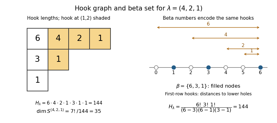
Pad $\lambda$ to $m$ rows and use the beta set of a partition ${\ell }_i={\lambda }_i+m-i$, so ${\ell }_1>\cdots >{\ell }_m\ge 0$ and ${\sum }_i{\ell }_i=n+d$, where $d=\left(\genfrac{}{}{0ex}{}{m}{2}\right)$. We prove the beta-set hook-product identity row by row. For $1\le j\le {\lambda }_i$, put $q_j=m+j-{\lambda }_j^{\prime }-1$; then $h_{ij}={\ell }_i-q_j$. The $q_j$ are distinct integers in $[0,{\ell }_i-1]$, and none equals a beta number. Indeed, if $k\le {\lambda }_j^{\prime }$ then ${\ell }_k\ge q_j+1$, whereas if $k>{\lambda }_j^{\prime }$ then ${\ell }_k\le q_j-1$. Exactly $m-i$ beta numbers lie below ${\ell }_i$, so the remaining ${\lambda }_i$ integers in that interval are precisely these $q_j$. ThereforeThis gives the equivalent Specht module dimension expression $f^{\lambda }=n!\Delta (\ell )/{\prod }_i{\ell }_i!$.

The standard Young tableaux of shape $\lambda$ form the dimension count for the Specht module. The largest entry $n$ must occupy a removable corner. Deleting it bijects tableaux with the disjoint union of standard tableaux of the shapes obtained by deleting a corner, provingSet a term to zero whenever $\lambda -e_i$ is not a partition: this includes equal adjacent rows and an attempted deletion from a zero row. The empty diagram has dimension $1$.

For an algebraic proof that the proposed formula has the same recurrence, establish the Vandermonde shift identityIts left side is an alternating polynomial in the $x_i$, because permuting the variables permutes the summands and changes the sign of every Vandermonde factor. It is therefore divisible by $\Delta (x)$. The quotient is symmetric in $x$ and homogeneous of total degree one in $(x,t)$, so has the form $a{\sum }_i{x}_i+bt$. At $t=0$, $a=1$. Differentiating in $t$ at zero and using the Euler theorem for homogeneous functions gives ${\sum }_i{x}_i{\partial }_i\Delta =d\Delta$, so $b=d$. This proves the identity as a polynomial identity, including repeated coordinates.

Take $x=\ell$ and $t=-1$. Since ${\sum }_i{\ell }_i=n+d$, it gives ${\sum }_i{\ell }_i\Delta (\ell -e_i)=n\Delta (\ell )$. For $n\ge 1$, this is exactlyThe summand is the proposed dimension for $\lambda -e_i$; if two beta numbers collide its Vandermonde is zero, and if ${\ell }_i=0$ its coefficient is zero, so no negative factorial is needed. For the empty partition, $\ell =(m-1,\dots ,0)$ and $\Delta (\ell )={\prod }_{k=0}^{m-1}k!$, giving initial value $1$. Induction now proves the hook-length formula from the tableau recurrence.

For the final sum, tuples with repeated coordinates contribute zero. Sorting each distinct nonnegative tuple with sum $\left(\genfrac{}{}{0ex}{}{m+1}{2}\right)$ gives one beta set of a partition of size $m$, since subtracting the staircase removes $\left(\genfrac{}{}{0ex}{}{m}{2}\right)$ from the sum. Conversely every partition of $m$, padded to $m$ rows, supplies exactly $m!$ ordered tuples, with the same squared summand. Hence the square-sum identity for shifted partition coordinates isThe middle equality uses the Artin–Wedderburn theorem for the group algebra and the complete classification of its simple modules by Specht modules. It explains why the last identity is a representation-dimension count rather than an accidental cancellation.

The space of test functions is $\mathcal{D}(\mathbb{R})=C_c^{\infty }(\mathbb{R})$: its elements are smooth functions with compact support. For a fixed compact set $K$, put ${\mathcal{D}}_K=\{\phi \in C^{\infty }(\mathbb{R}):\mathrm{supp}\phi \subset K\}$ and use the seminorms $p_m(\phi )={\max }_{0\le j\le m}\Vert {\phi }^{(j)}{\Vert }_{\infty }$. The space of test functions carries the usual test-function inductive limit topology of these spaces. In particular, a sequence converges precisely when its supports eventually lie in one compact set and every derivative converges uniformly. Thus ${\phi }_j\to \phi$ means that a common $K$ contains their supports and $p_m({\phi }_j-\phi )\to 0$ for every $m$.

A distribution is a continuous linear functional on this space of test functions, and ${\mathcal{D}}^{\prime }(\mathbb{R})$ denotes their space. We use complex-linear, bilinear pairings $⟨u,\phi ⟩$. Equivalently, for every compact set $K$ there are $C_K$ and a nonnegative integer $m_K$ such thatThe usual weak convergence of distributions is $u_j\to u$ if $⟨u_j,\phi ⟩\to ⟨u,\phi ⟩$ for every test function. This specifies the convergence used below; it does not require convergence in any norm.

The distributional derivative is defined byThe derivative map sends ${\mathcal{D}}_K$ continuously to itself, with $p_m({\phi }^{\prime })\le p_{m+1}(\phi )$. The preceding continuity estimate therefore proves that $u^{\prime }$ is again a distribution. This definition extends the ordinary derivative of a smooth function, by integration by parts.

Choose the translation of a distribution convention ${\tau }_{h}f(x)=f(x-h)$. Its action on a test function isFor fixed $h$, the translated test functions have translated compact support and unchanged derivative sup norms, so this defines a distribution. For the differentiability of distribution translations, apply the Taylor theorem in integral form:All supports lie in one slightly enlarged compact set for $|h|\le 1$, and the same identity for every derivative proves uniform convergence. The continuity of $u$ now givesThe minus sign in the translation parameter is necessary for this convention.

For (a), choose a test function $\eta$ with $\int \eta =1$. If $\int \psi =0$, then $F(x)={\int }_{-\infty }^x\psi (s)ds$ is a test function, since the zero integral makes it vanish beyond both ends of the compact support. If $u_1^{\prime }=0$, then $⟨u_1,\psi ⟩=⟨u_1,F^{\prime }⟩=0$. Decompose $\phi =(\int \phi )\eta +\psi$ to obtainConversely, these constant regular distributions have zero distributional derivative. This also proves the general fact that a distribution with zero derivative is constant.

For (b), choose a cutoff function $\rho$ equal to one near zero. Every test function decomposes asThe quotient extends as a smooth function at zero, and it has compact support. If $x{u}_2=0$, the definition of multiplication of a distribution by a smooth function gives $⟨u_2,\phi ⟩=⟨u_2,\rho ⟩\phi (0)$. Conversely, $x{\delta }_0=0$. Thus the kernel of multiplication by a coordinate is exactlyIn particular, derivatives of the Dirac delta distribution are not additional solutions: $x{\delta }_0^{\prime }=-{\delta }_0$.

Now write $D=d/dx$ and $P(z)=-z^n+{\sum }_{j=0}^{n-1}{a}_j{z}^j$, where $n\ge 1$. The characteristic roots of a constant-coefficient differential equation are the distinct roots of a polynomial ${\lambda }_1,\dots ,{\lambda }_r$ of $P$, with multiplicities $m_1,\dots ,m_r$. The distributional regularity of a constant-coefficient ordinary differential equation can be proved without assuming regularity in advance. Put $q_j(z)=(z-{\lambda }_j{)}^{m_j}$ and $Q={\prod }_j{q}_j=-P$. Since the $q_j$ are coprime polynomials, polynomial division and Bezout identity give polynomials $b_j$ such thatFor example, invert $Q/q_j$ modulo $q_j$, sum the resulting expressions, and absorb a remaining multiple of $Q$ into one coefficient. For $P(D)v=0$, the kernel decomposition for coprime polynomials therefore givesThe Leibniz rule for multiplication of a distribution by a smooth function implies $D^{m_j}(e^{-{\lambda }_{j}x}{v}_j)=0$. Repeatedly using a distribution with zero derivative is constant shows that a distribution with $m$th derivative zero is a polynomial of degree at most $m-1$: subtract the polynomial primitive of its constant $(m-1)$st derivative, and induct on $m$. Consequently the most general exponential polynomial solution of a constant-coefficient differential equation isEvery displayed term is annihilated by $P(D)$, so all coefficients are allowed. For the linear independence of these $n$ functions, on a relation, apply ${\prod }_{i\ne j}(D-{\lambda }_i{)}^{m_i}$; on $e^{{\lambda }_{j}x}$ times a polynomial of degree less than $m_j$, each remaining factor acts invertibly on that polynomial space. Hence the $j$th polynomial must vanish. Every distributional solution is an analytic function, and in particular a classical solution. For real coefficients and real-valued distributions, take complex conjugate coefficients at conjugate characteristic roots of a constant-coefficient differential equation, or equivalently use the corresponding real sine and cosine forms.

For the last equation, the operator is $xP(D)$: the coordinate multiplies the result of differentiation. The kernel of multiplication by a coordinate says precisely thatChoose the retarded fundamental solution of a constant-coefficient ordinary differential operator $E=Hw$, where $H$ is the Heaviside function and $w$ is the analytic solution of $P(D)w=0$ withSuch $w$ exists uniquely by the elementary initial value problem for a constant-coefficient ordinary differential equation; alternatively the residue construction in the next solution gives it explicitly. The distributional jump formula for a Heaviside product isIt follows by induction from $D(Hw)=H{w}^{\prime }+w(0){\delta }_0$, using integration by parts. With the chosen initial derivatives, every lower-order jump term vanishes and the leading coefficient $-1$ gives $P(D)E={\delta }_0$. Subtracting $CE$ reduces the last equation to the homogeneous one. Thus the coordinate-degenerate constant-coefficient differential equation has exactly the solutionsThere are $n+1$ independent constants. For $n\ge 2$, derivatives through order $n-2$ match at zero, while the derivative of order $n-1$ may jump; for $n=1$, the function itself may jump. An arbitrary distribution concentrated at zero cannot be added, because its image under the nonzero leading derivative would contain a nonvanishing highest derivative of the Dirac delta distribution.

The Malgrange–Ehrenpreis theorem states that every nonzero constant-coefficient linear differential operator on Euclidean space has a distributional fundamental solution. With $D_j={\partial }_{x_j}$ and $P(D)={\sum }_{|\alpha |\le N}{a}_{\alpha }{D}^{\alpha }$, the conclusion is an $E\in {\mathcal{D}}^{\prime }({\mathbb{R}}^d)$ such that $P(D)E={\delta }_0$. If $N=0$, simply take $E=a_0^{-1}{\delta }_0$; hence assume $N\ge 1$.

We construct a Hörmander staircase in frequency space. The highest-degree homogeneous part $P_N$ is not identically zero on real vectors, since a polynomial vanishing on all real vectors has all coefficients zero. After an orthogonal transformation of coordinates, we can arrange that $P_N(e_1)\ne 0$. Thus, for each real ${\xi }^{\prime }\in {\mathbb{R}}^{d-1}$, the polynomialhas degree $N$ in $z$ and the same nonzero leading coefficient $b=i^N{P}_N(e_1)$, independent of ${\xi }^{\prime }$. This constant leading coefficient of a polynomial is what makes a uniform staircase possible.

For a fixed ${\xi }^{\prime }$, factor $p(z,{\xi }^{\prime })=b{\prod }_{\nu =1}^N(z-z_{\nu })$, counting repeated roots of a polynomial. Consider the $N+1$ heights $h_j=3j$, $j=0,\dots ,N$. A given root has imaginary part within distance less than one of at most one of these heights. By the pigeonhole principle, some height avoids every root, and thenThis is finite-height polynomial root avoidance. Root labels need not be chosen continuously or even measurably. Instead define the closed setsContinuity in $s$ extends the inequality from rational $q$ to every real $s$. These Borel sets partition ${\mathbb{R}}^{d-1}$. The Hörmander staircase assigns the horizontal contour $s+i{h}_j$ over $A_j$; its height is bounded by $3N$, and the denominator has the uniform lower bound $|b|$. For $d=1$, the transverse space is a single point and only one horizontal contour is needed.

Use the Fourier transform convention $\hat{\phi }(\zeta )=\int e^{-ix\cdot \zeta }\phi (x)dx$, with inverse factor $(2\pi {)}^{-d}$. Define the candidate fundamental solution of a linear differential operator byFor a test function supported in a fixed compact set $K$, Fourier decay in a bounded complex strip gives, for any integer $M$,Indeed, this is the real Fourier transform of $e^{-h_j{x}_1}\phi (x)$ with reversed frequency, and repeated integration by parts with $(1-\Delta {)}^M$ proves the estimate. Taking $2M>d$ and using the denominator bound proves absolute convergence and a continuity estimate on ${\mathcal{D}}_K$. Thus $E$ is a distribution; no unsupported interpretation of a divergent inverse Fourier transform is being used.

For its distributional derivatives, the formal transpose of a differential operator is $P(-D)$. Sinceapplying $P(D)$ cancels the denominator. For each fixed ${\xi }^{\prime }$, the numerator is an entire function of $z$. The Cauchy integral theorem, applied to a rectangle between the lines $\mathrm{Im}z=0$ and $\mathrm{Im}z=h_j$, givesThe two vertical edges tend to zero by the same bounded-strip decay. The resulting contour deformation is performed separately for each transverse frequency, so discontinuities of the staircase height introduce no additional boundary terms. Absolute convergence permits integration over the partition $A_j$. The Fourier inversion theorem then yieldsThis proves the Malgrange–Ehrenpreis theorem. Undoing the orthogonal change of coordinates gives the fundamental solution of a linear differential operator for the original operator; the Dirac delta distribution is unchanged by that change of coordinates.

For a one-dimensional operator $L=P(D)$ of degree $N\ge 1$, with leading coefficient $a_N$, we may choose the single staircase contour below every pole. Take $\gamma >\max \{\mathrm{Re}\lambda :P(\lambda )=0\}$ and integrate on $\mathrm{Im}\zeta =-\gamma$. The corresponding formula is the Bromwich contour version of the construction above, after putting $\lambda =i\zeta$. Its poles all lie above the frequency contour. For $x<0$, close that contour downwards; the exponential function $e^{ix\zeta }$ decays and there are no enclosed poles. For $x>0$, close upwards, where the exponential function again decays, and apply the residue theorem. The bound $1/P(i\zeta )=O(|\zeta {|}^{-N})$ justifies the large arcs, including $N=1$ by the Jordan lemma away from their endpoints. Thus away from $x=0$ the retarded fundamental solution is $H(x)u(x)$, whereThe sum is over distinct roots of a polynomial, with the residue including the whole multiplicity. For simple characteristic roots of a constant-coefficient differential equation, it reduces to $u(x)={\sum }_{\lambda }{e}^{\lambda x}/P^{\prime }(\lambda )$. Repeated roots give exponential polynomial solutions of a constant-coefficient differential equation through differentiation of $e^{zx}$.

To establish the equality also at the origin, rather than leave a possible point-supported term undecided, verify the distributional jump formula for a Heaviside product. The residue expression is an entire function of $x$, andIts initial derivatives areThese identities follow by integrating over a large circle: for $j\le N-2$ the integrand is $O(|z{|}^{-2})$, whereas for $j=N-1$ its coefficient of $z^{-1}$ is $a_N^{-1}$. The distributional jump formula for a Heaviside product therefore gives $L(Hu)={\delta }_0$. Moreover, since $e^{-\gamma x}Hu$ is a tempered distribution, its Fourier transform satisfiesThere are no real zeros of this polynomial, so its reciprocal is the transform. This is exactly the shifted-contour construction, proving equality there as a distribution as well. HenceThe sign of $a_N$ matters: for the operator in the preceding solution, $a_N=-1$ and the last initial derivative is $-1$.

Let $m$ be a positive integer and let the trigonometric polynomial $t_n$ have frequencies only in $[-n,n]$. For every $j\ge n$, its Fourier partial sum is the polynomial itself: $s_j(t_n)=t_n$. Every term in the defining average of the de la Vallée Poussin sum therefore equals $t_n$, givingThis is exact reproduction of the degree-at-most-$n$ trigonometric polynomials, irrespective of the positive averaging length $m$.

Put $r=k-1$. The linear-reproduction request requires $k\ge 2$, which we use for that final step. Since ${\psi }_i={\omega }_i/r!$, the useful normalized Marsden dual functional isThere is no further factor $1/r!$ outside this sum: it has already been included in ${\psi }_i$.

To derive the formula directly from Marsden's identity, Taylor's theorem for the polynomial $p$ around the arbitrary point $x$ givesOn the other hand,Differentiate Marsden's identity $r-j$ times in $x$, multiply by $(-1{)}^j{p}^{(j)}(x)/r!$, and sum over $j$. The left side becomes $p(t)$, while the right side becomesOnly finite sums and derivatives of polynomials are involved.

Independence of the auxiliary point does not require an assumption about uniqueness of an expansion. Differentiate the formula for ${\lambda }_i$ itself:The first summand at $j=r$ and the second at $j=0$ vanish because both polynomials have degree at most $r$. All remaining terms cancel after shifting the index by one. Therefore ${\lambda }_i(p)$ is a constant in $x$, and it is visibly a linear functional of $p$.

For $p(t)=a+bt$, only $j=0,1$ remain. The leading two coefficients of the monic knot polynomial giveIt follows thatSubstituting into the expansion proveson the basic knot interval. Thus the Greville abscissae are exactly the sampling coefficients that reproduce linear polynomials; the constant case also gives the subpartition of unity for B-splines with equality on this interval.

Write the strictly increasing local spline knots as $u_j=t_{i+j}$, $0\le j\le k$. The explicit formula for a divided difference givesEach summand is a truncated power function of $t$: it is a polynomial on either side of its knot $u_j$, and for $k\ge 2$ is globally $C^{k-2}$. Hence $M_i$ is a piecewise polynomial function of degree at most $k-1$, with these spline knots and at least this global smoothness.

For $t\ge u_k$, all summands vanish. For $t<u_0$, all knot values agree with those of the ordinary polynomial $(s-t{)}^{k-1}$ in the divided-difference variable $s$. Its order-$k$ divided difference is zero, because its degree is less than $k$. Thus $M_i$ also vanishes to the left of $u_0$.

The closed support is exactly the indicated interval, rather than merely contained in it. For $u_0<t<u_1$, subtracting the omitted $j=0$ term from the zero divided difference of $(s-t{)}^{k-1}$ givesFor $u_{k-1}<t<u_k$, only the last truncated-power term survives, givingThere are therefore nonzero values arbitrarily close to either endpoint, provingAt each simple knot, the $(k-1)$st derivative has a nonzero jump from exactly one truncated-power summand, so this is also the exact global smoothness. For order $k=1$, the function is instead the normalized interval indicator; there is no assertion of classical continuity, and the notation $C^{k-2}$ is only the customary formal spline smoothness notation. This distinction is part of simple-knot B-spline regularity.