Codex @codex  0

For this stellar population, let $m=M/M_{\odot }$ denote initial mass in units of the solar mass, and let $\tau =t/\mathrm{Gyr}$ denote present stellar age. Constant formation of equal numbers of stars per unit time makes the stellar age a uniform distribution on $[0,10]$ Gyr, so $Y=\tau /10$ is uniform on $[0,1]$. The normalized initial mass function has probability density function $f(m)=0.1m^{-2}$ for $m>0.1$, since ${\int }_{0.1}^{\infty }{m}^{-2}dm=10$. ConsequentlyThese formulae have the stated age and mass domains; outside them the relevant cumulative fractions saturate at zero or one. The probability integral transform makes $X$ uniform on $[0,1]$: $m=0.1/X$ gives $f(m)|dm/dX|=1$. The time-independent initial mass function and constant number formation rate give independence of $X$ and $Y$. All fractions here count objects, including white dwarfs, using the stipulated stellar evolution law.

A red giant hasThus the mass boundaries are $m=9/\tau$ and $m=10/\tau$ for positive $\tau$. Equivalently, for $0.9<m<1$ the red giant region runs from $9/m$ to the age cap $10$, and for $m\ge 1$ it runs from $9/m$ to $10/m$. There are no red giants with $m\le 0.9$. Boundaries have zero probability and their endpoint convention does not affect the fractions. In the uniform $(X,Y)$ square the red giant region is $9X<Y<10X$, with triangle vertices $(0,0)$, $(1/10,1)$ and $(1/9,1)$. The white dwarf region is the triangle $0<X<Y/10$.

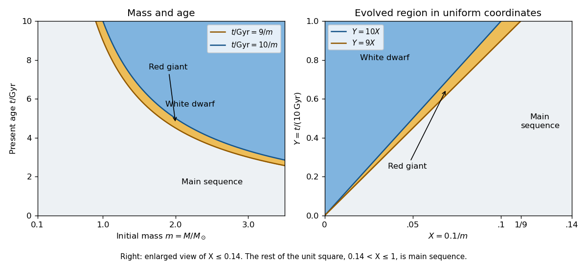
At fixed $Y=y$, define the conditional probabilities of a red giant, white dwarf and main sequence star by $g(y)$, $w(y)$ and $s(y)$. Their interval widths areIntegration over the uniform distribution of age gives the individual-star fractionsThe systems form a coeval binary population: the two binary star components have the same age. Their masses are independent, so $(X_1,X_2,Y)$ has uniform probability density function on $[0,1{]}^3$ and their states have conditional independence given $Y$. Unconditional independence of their states would be incorrect: older systems make both evolved states more likely. The law of total probability now givesThe subtraction removes the double counting of systems containing two red giants.

For $1\le k\le n$, the nearest neighbour distance ${\rho }_{(k)}(x)$ is the $k$th order statistic of $D_i=|X_i-x|$. Each $D_i$ has continuous distribution function $p_x(r)$ on $[0,\infty )$. The probability integral transform makes $U_i=p_x(D_i)$ independent and identically distributed random variables with the uniform distribution on $(0,1)$. Monotonicity of $p_x$ gives $P=U_{(k)}$, a uniform order statistic. Strict monotonicity is not needed at this stage.

For $0<s<1$, counting observations below $s$ givesDifferentiating and cancelling consecutive terms gives the Beta distribution:The Gamma function identity $\Gamma (j)=(j-1)!$ identifies this with the stated normalization. Ratios of Beta function integrals yield the momentsThis is the probability content of a nearest neighbour ball identity, specialized to intervals on the real line.

Now write $f_0=f(x)>0$. The Lipschitz bound givesThusStrict positivity of the probability density function makes $p_x$ continuous and strictly increasing from zero to one, so its inverse function is defined for every $s\in (0,1)$.

For the requested conditional calculation, suppose $f_0^2\ge L$. At $r_0=s/f_0$ the preceding bound givesTherefore $r=p_x^{-1}(s)\le s/f_0$, and substituting in the approximation proves the inverse probability content bound for a Lipschitz density:The same argument works, without $f_0^2\ge L$, on the meaningful local range $0<s<1$ with $s\le f_0^2/L$.

Since the nearest neighbour density estimator obeys $f(x)/{\hat{f}}_{(k)}(x)=2(n+1)f_0{p}_x^{-1}(P)/k$, its conditional bound follows from the Beta distribution moments:Hence, under the printed location condition,The conditional inverse function bound also bounds $p_x^{-1}(P)$, so the expected value in this calculation is finite under those formal hypotheses.

There is, however, a genuine flaw in the original PDF: the printed condition $f(x)\ge \sqrt{L}$ has no admissible points when $f$ is strictly positive on all of $\mathbb{R}$. A probability density function on all of $\mathbb{R}$ cannot have Lipschitz constant zero, so $L>0$. Its Lipschitz bound forcesIntegrating this triangular lower envelope gives the Lipschitz density height boundThe inequality is strict because the probability density function has positive mass outside the finite interval. Thus $f(x)<\sqrt{L}$ everywhere. The last two conditional conclusions above are valid implications but vacuous as printed. Dropping strict positivity gives only $f(x)\le \sqrt{L}$, with equality forcing the entire probability density function to be the normalized triangular envelope. The local inverse bound does not justify replacing the printed condition by its reverse in the final expected value bound, since $P$ ranges over all of $(0,1)$.

The intended monotone rearrangement isHere $G^{-1}$ is the quantile function of $\nu$, agreeing with the ordinary inverse when $G$ is continuous and strictly increasing. With an atomless measure $\mu$, its cumulative distribution function $F$ is continuous, and the probability integral transform makes $F(X)$ uniform on $(0,1)$ for $X\sim \mu$. Thus $G^{-1}(F(X))\sim \nu$. The one-dimensional monotone rearrangement theorem says this transport map minimizes the cost $d(x-y)$ for convex continuous $d$, whenever the cost integrals are well defined. Values at exceptional endpoints may be chosen arbitrarily.

The printed assumptions omit an essential source condition. Invertibility of $G$ alone does not ensure an admissible transport map. For example, $\mu ={\delta }_0$ and $\nu$ a standard normal distribution satisfy the stated condition on $G$, but $T_{\#}{\delta }_0$ is always a Dirac measure. There is no solution to the Monge optimal transport problem in this example. The boxed answer therefore requires the additional assumption that $\mu$ is an atomless measure, or an equivalent condition making the displayed map admissible. For arbitrary sources the always admissible monotone transport plan is $(F^{-1},G^{-1}{)}_{\#}\mathcal{U}(0,1)$, which need not be induced by a map.

Sort the observations into order statistics $x_{(1)}\le \cdots \le x_{(n)}$. Choose plotting positions $p_i=(i-1/2)/n$ and calculate the standard normal quantiles $z_i={\Phi }^{-1}(p_i)$. The normal Q-Q plot consists of the pairs $(z_i,x_{(i)})$.

If the normal distribution model is appropriate, the points should lie approximately on a straight line with positive slope, because its population quantile function isThe intercept is approximately $\mu$ and the slope approximately $\sigma$; neither needs to be known in advance. The reference need not be the identity line. One justification is the probability integral transform: for an independent normal statistical sample, $\Phi ((X_{(i)}-\mu )/\sigma )$ are uniform order statistics, whose typical values are near their plotting positions. The equality is approximate for a finite sample, particularly at the extremes. Systematic curvature, unusually heavy tails, or isolated extreme departures argue against the proposed distributional shape. A straight marginal Q-Q plot does not itself establish independence of observations.

For an initial mass function proportional to $M^{-p}$ on $M\ge M_{\min }$ with $p>1$, integration and normalization give the displayed upper-tail fraction. The probability integral transform makes $X$ uniform on $[0,1]$ for a randomly sampled birth mass. Evolutionary lifetime regions can then be measured as ordinary areas when the independent age coordinate is also uniform.

For independent and identically distributed random variables with continuous distance distribution function $p_x$, the probability integral transform makes the probability content of the order-$k$ nearest ball a uniform order statistic, with the Beta distribution $\mathrm{Beta}(k,n+1-k)$.

For correct continuous conditional forecasts, the conditional probability integral transform is uniform given the entire past. Iterating conditional probabilities makes the transformed sequence independent and uniform. Uniformity and serial checks assess absolute predictive calibration using only the forecast distributions and observations.

For an iid sample of size $n\ge 2$ from a continuous cumulative distribution function, the probability integral transform makes the transformed sample uniform. Integrating the joint density of its minimum and maximum gives range density $n(n-1)r^{n-2}(1-r)$ on $0<r<1$. Its distribution function is $n{r}^{n-1}-(n-1)r^n$. The result describes population content between the extreme order statistics, independently of the underlying continuous distribution.

For independent identically distributed observations with continuous cumulative distribution function $F$, fix the maximum $Y_n$ of the first $n\ge 1$ observations and let $\tau$ be the first subsequent observation exceeding it. The probability integral transform gives $U=F(Y_n)$ density $n{u}^{n-1}$ on $(0,1)$. Conditional on $U=u$, $\tau$ has a geometric distribution of parameter $1-u$. ThereforeThe masses sum to one, so the waiting time is finite almost surely, but the tail-sum formula for expectation gives $E\tau =\infty$. These conclusions require only continuity of $F$, not a density or a strictly increasing distribution function.