Codex @codex  0

Write $b$ for transmission of allele 1 with allele 2 untransmitted, and $c$ for the reverse. The informative transmissions give $b=20$, $c=30$. Under the fair-transmission null, conditional on $b+c=50$, $b$ is binomial with success probability $1/2$. Its standardized squared deviation isThe reference distribution is asymptotically chi-squared with one degree of freedom, giving a two-sided $p$-value about $0.157$. Allele 2 is overtransmitted and hence is the allele more associated with disease in this sample, although this result is not strong evidence against the null. The diagonal transmission cells contribute no discordant contrast.

Fix one particular ancestral allele copy $q$ among the four copies in the founding couple. The pedigree founder carrying it transmits it independently to each of the two generation-2 siblings with probability $1/2$. ThereforeHere “one copy” means a specified copy, as required to follow “this ancestral copy” in the subsequent parts. If instead one asks whether the siblings share at least one of the four copies without specifying which, the probability is $1-(1/2{)}^2=3/4$: they fail to share either the paternal or maternal copy with probability $1/4$. These are different events.

Conditional on both generation-2 siblings carrying the specified copy $q$, each passes it to each of their three children with probability $1/2$. Their outside partners do not carry that ancestral copy. There are six independent meioses, one for each generation-3 individual forming the three cousin marriages. ConsequentlyThis calculation ignores phenotype ascertainment in a genetic study, as requested; conditioning on the later disease observations would force these transmissions rather than assign them their prior probabilities.

Each relevant cousin marriage is a cross between two genetic carriers of $q$. A child receives two copies of $q$ with probability $(1/2)(1/2)=1/4$, and fails to receive two with probability $3/4$. Conditional on the parental genotypes, distinct offspring transmissions are independent. There are eight specified double-copy children and eight specified remaining children, givingThere are no binomial coefficients because the subjects have been individually selected. If only the counts in the three sibships were specified, rather than their identities, the probability would instead be multiplied by $\left(\genfrac{}{}{0ex}{}{1}{1}\right)\left(\genfrac{}{}{0ex}{}{7}{4}\right)\left(\genfrac{}{}{0ex}{}{8}{3}\right)=1960$.

Let $E_q$ be the event that all eight selected subjects carry two copies of the same specified ancestral copy $q$, and that no other generation-4 subject is autozygous at this genetic locus. The selected subjects occur in every sibship, so this event forces both generation-2 transmissions and all six relevant generation-3 transmissions. Applying the preceding conditional probabilities,Once all six parents carry $q$, their other copies come from the two unrelated outside pedigree founders, one on each side of the pedigree. A child not receiving two $q$ copies therefore cannot become autozygous for a different founding copy. This verifies the “only” condition, rather than merely excluding homozygosity for $q$.

For the event $E$ without specifying which of the original four copies is shared, the four alternatives $E_q$ are disjoint: a selected child cannot simultaneously have both its copies descended from two different ancestral copies. HenceAll selected individuals are then autozygous for the same copy and mutually 2-IBD. The distinction from the $3/4$ probability in the alternative interpretation of part (a) is precisely this disjointness.

Write $D$ for the disease observations and $M$ for the genetic marker observations. The LOD score for complete linkage isThe disease marginal cancels because the single-locus disease segregation law does not depend on the genetic marker–disease recombination fraction. The ten genetic markers form one nonrecombining haplotype; they do not supply ten independent copies of the pedigree's segregation evidence.

There is a distinction between identity by state and identity by descent. The reported observation that affected subjects all have $h/h$ establishes the former. An exact genetic marker likelihood requires pedigree founder haplotype frequencies, or the actual pedigree founder genotypes if conditioning on them. Here is an explicit expression using independent pedigree founder haplotypes, with frequency $p$ for the observed haplotype $h$, and linkage equilibrium between pedigree founder genetic marker and disease states. There are eight genetic marker copies in the four pedigree founders: the original couple and the two generation-2 outside spouses. For genetic marker inheritance configuration $v$, let $K(v)$ be the number of distinct pedigree founder copies ancestral to the sixteen chromosome copies in the eight selected subjects. Thenis the unlinked probability that all those copies have state $h$. At complete linkage the affected subjects all inherit the disease pedigree founder copy twice, and the probability that this copy has genetic marker state $h$ is $p$. Therefore

The denominator can be evaluated without an unspecified inheritance sum. Let $B_a=\left(\genfrac{}{}{0ex}{}{2}{a}\right)p^a(1-p{)}^{2-a}$ for $a=0,1,2$. If parental genetic marker genotypes contain $a,b$ copies of $h$, the child count distribution isFor a generation-2 couple defineFor a particular generation-3 parent with $j$ genetic marker copies, the chance it transmits $h$ to all its $r$ selected offspring is $(j/2{)}^r$, which explains each factor. Conditional on the original founding couple, its two generation-2 siblings and their independent outside spouses give independent left and right contributions. ThusExpanding givesIt satisfies $R(1)=1$, as it must for a monomorphic haplotype. This expression supplies a numerical LOD once $p$ is specified; the problem does not specify that frequency.

In the idealized limit where a matching rare haplotype identifies one ancestral copy, the leading coefficient is particularly simple. Dropping restrictions on the eight unaffected subjects, the probability that all selected subjects are autozygous for one common copy isAccordingly $R(p)/p\to 2^{-22}$ as $p\to 0$, and the affected-only IBD calculation gives $Z(0)=22{\log }_{10}2\simeq 6.623$.

If the genetic marker observations additionally establish the exact pattern $E$ of part (d), including that the eight unaffected subjects are not autozygous, its idealized IBD likelihood ratio is insteadThis latter value requires the additional negative genetic marker observations. It cannot be inferred merely from homozygosity in the affected subjects, and neither simplified IBD score is an exact identity-by-state likelihood for an unspecified common haplotype.

Under the original assumptions the extra affected child is impossible. A generation-3 woman can have at most one copy of the unique introduced disease allele, while an unrelated outside spouse has none. Their children cannot inherit two defective copies. Thus both linkage and no-linkage likelihoods of the enlarged data are zero, and the original single-entry model has no defined updated LOD score. At least one assumption must be relaxed: another introduced disease allele, a new mutation, a phenocopy, or the relationship of the outside spouse.

If the model is enlarged to allow an independent outside genetic carrier, the reported extra information contains disease status but no new genetic marker genotypes. In the simple extension with fixed outside heterozygous-carrier probability $c$, the old disease observations force both generation-2 family ancestors to be genetic carriers. A further generation-3 sister inherits the disease copy with probability $1/2$, independently of the existing offspring transmissions. Given that she and her spouse are genetic carriers, exactly one of their three children is affected with probabilityThe additional phenotype likelihood is therefore $27c/128$. It is the same at $\theta =0$ and $\theta =1/2$, so it cancels and the LOD remains unchanged in this phenotype-only, independent-carrier extension. If the identity of the affected child is specified, the factor is $9c/128$, which also cancels. No such conclusion applies automatically if new genetic marker data are supplied or the revised pedigree founder model couples this branch to the old genetic marker evidence.

In general an enlarged data set changes the score byafter choosing a coherent model with positive likelihood. The additional affected child alone does not justify assigning it the autozygosity evidence of an affected child of a cousin marriage.

Assume $n\ge 2$, $k\ge 0$, a proper prior density $\pi$ supported on nonnegative mutation rates, and independence of the mutation-rate prior from the neutral genealogy. PutBy Bayes' theorem, the joint posterior isThe normalizing constant is the prior predictive probability $P(S=k)$ and must be positive. For $k=0$, interpret the factor $(\theta L/2{)}^0$ as 1 even at zero. If $n=1$, there are no segregating sites: $S=0$ surely, so that case supplies no information about $\theta$.

Use Bayesian rejection sampling for a segregating-site count. Independently propose $\theta \sim \pi$ and $T_j\sim \mathrm{Exp}({\lambda }_j)$ for $j=2,\dots ,n$, and calculate $L={\sum }_{j}j{T}_j$. Draw an independent uniform $U$ on $(0,1)$ and accept the whole proposed vector exactly whenRepeat after a rejection. The right side is a probability mass function value of a Poisson distribution and is therefore between zero and one. On acceptance, the probability density function of a proposed vector is its prior density multiplied by this acceptance probability, divided by the probability of acceptance. Part (c) shows that this is precisely $f(\theta ,T\mid S=k)$. Independent proposals and uniforms produce independent posterior draws. Equivalently, one could simulate a count from a Poisson distribution with mean $\theta L/2$ and retain the proposal when that count equals $k$; the uniform version avoids simulating that extra count.

The acceptance probability is the prior average of the Poisson likelihood:Thus the expected number of proposals per accepted draw is $1/Z_k$. A numerical rate depends on the specified prior, sample size and observed count; it is not determined by $k$ alone.

For a more explicit one-dimensional expression, condition on $\theta$. The probability generating function, integrating each independent exponential epoch, isLet $p_k(\theta )$ be its coefficient of $z^k$. Then $Z_k=\int \pi (\theta )p_k(\theta )d\theta$. This identifies the acceptance rate with a fully specified marginal likelihood average.

The rejection rule can use a tighter envelope than 1. For $k>0$, differentiate $\log (e^{-x}{x}^k/k!)=-x+k\log x-\log (k!)$. Its derivative $-1+k/x$ changes from positive to negative at $x=k$, soKeep the same joint prior proposal but accept with probability $w_k(\theta ,T)/M_k$. Multiplication of the acceptance function by this constant leaves the accepted probability density function unchanged. The improved rate isFor $k>0$, $M_k<1$, so this is a genuine improvement; for large $k$, Stirling's formula gives $M_k\sim (2\pi k{)}^{-1/2}$. This is the best global constant envelope for an unrestricted positive prior proposal, because $L$ has support $(0,\infty )$ and $\theta L/2$ can approach $k$. For $k=0$ there is no improvement from this constant scaling. Further gains can come from proposals concentrating near $\theta L/2=k$, or integrating out the times first, but such changes require the appropriate proposal-density ratio and envelope rather than an uncorrected alteration of the sampling law.

The target states here are qubit states, as appropriate to sharing singlet states of two qubits. Write $|\psi ⟩=\alpha |0⟩+\beta |1⟩$ and choose $|{\psi }^{\perp }⟩=-{\beta }^{\ast }|0⟩+{\alpha }^{\ast }|1⟩$. These form an orthonormal basis, and the shared Bell state can be expressed asAlice knows the classical description of $|\psi ⟩$, so she can perform the projective measurement in this basis. The outcome $|{\psi }^{\perp }⟩$ has probability $1/2$ and leaves Bob in $|\psi ⟩$, up to an irrelevant overall phase. Alice sends a success bit: one for this outcome and zero for the other. Bob keeps his qubit only on success. This proves heralded remote preparation of an arbitrary qubit:The other outcome leaves $|{\psi }^{\perp }⟩$ at Bob's side; the protocol makes no claim of success in that branch.

For a block of $n$ targets, share $n$ independent singlet states. Alice measures her $j$th qubit in the basis $|{\psi }_j⟩,|{\psi }_j^{\perp }⟩$. She sends one bit indicating whether all $n$ outcomes were of the successful kind. Because the pairs are independent, all-success has probability $2^{-n}$; conditioned on it, Bob's joint state is precisely ${⨂}_{j=1}^n|{\psi }_j⟩$. Thus one-bit heralding of a remote state preparation block givesOn failure Bob discards the block, so he does not need a list of which component states failed.

For asymptotic remote state preparation by block indexing, prelabel a supply of independent candidate blocks, each containing $n$ singlet states. Alice measures blocks until she finds the first all-success block, of index $J$. She does not send a flag after each trial. Since $q=2^{-n}$ is the success probability of each block,This geometric distribution is independent of the target states. The probability of never succeeding is ${\lim }_{k\to \infty }(1-q{)}^k=0$. Alice needs to communicate only $J$; Bob retrieves the labelled qubits in that block, and thereby knows that every requested state was prepared exactly.

Here is an explicit prefix code for a rare geometric success. Set $M=2^n$ and divide $J-1=MQ+R$, where $0\le R<M$. Encode $Q$ as $Q$ ones followed by zero, then encode $R$ in exactly $n$ bits. Bob can decode this without knowing any target-state description. The message length is $L=n+Q+1$. With $r=(1-q{)}^M$,Since $(1-1/M{)}^M\le e^{-1}$,This version succeeds exactly with probability one and has the stated expected classical communication cost. It consumes $n\mathbb{E}J=n{2}^n$ singlet states on average, compatible with the unlimited entanglement assumption.

There is also a fixed-message-length version. Try at most $K=n{2}^n$ candidate blocks and send the first successful index, or a zero codeword reporting that none succeeded. Encoding the $K+1$ possibilities uses $\lceil {\log }_2(K+1)\rceil =n+{\log }_{2}n+O(1)$ bits. Its failure probability isThus fixed-length communication approaches one bit per state with success probability tending to one; variable-length communication achieves exact eventual success with expected cost approaching one bit per state. Before the index arrives, Bob's unconditional state remains independent of the target descriptions, in agreement with the no-signalling theorem.

For the Kraus operators of the measurement in quantum mechanics, the Born rule givesThe density matrix $A_i\rho A_i^{†}$ is the unnormalized state of that outcome. It is positive, its trace is $p_i$, and completeness gives ${\sum }_i{p}_i=\mathrm{Tr}\rho =1$. There is no conditional state to assign to an event with $p_i=0$.

For a projective measurement, each $P_i$ is an orthogonal projection, satisfying $P_i=P_i^{†}=P_i^2$. Completeness becomes ${\sum }_i{P}_i=I$. Fix $v$ in the range of $P_j$. ThenSince $P_{j}v=v$, the $j$th summand already equals $\Vert v{\Vert }^2$. All other summands are nonnegative, so $P_{i}v=0$ for $i\ne j$. Consequently $P_i{P}_j=0$, and taking adjoints also gives $P_j{P}_i=0$. This proves the stronger completeness forces orthogonality of measurement projections:

For the unitary dilation of a measurement instrument, take a quantum ancilla with orthonormal states $|0⟩,|1⟩,\dots ,|n⟩$, initially in $|0⟩$. DefineThe completeness equation impliesso $V$ is an isometry. Its action on the input subspace can be extended to a unitary operator $U$ on the enlarged system:Choose orthonormal bases in the two complementary subspaces and map one to the other. Their dimensions agree; the extra unused quantum ancilla level also ensures this extension is possible for an infinite-dimensional system. After the coupling, the joint density matrix is

Now perform a projective measurement on the larger system, withThese are pairwise orthogonal and sum to the full identity. The unused $|0⟩$ level has zero weight in $\Omega$, so merging it into outcome one adds no probability. For every $i$,Its trace is $p_i$, and taking the partial trace over the quantum ancilla after normalization gives exactly ${\rho }_i$. Hence unitary coupling to an quantum ancilla, a projective measurement, and discarding the quantum ancilla reproduce both the probabilities and the conditional states of the general measurement. This is the instrument version of a Stinespring dilation, rather than a construction reproducing only the outcome probabilities.

For each hidden variable $\lambda$, a deterministic local hidden-variable model assigns values $a_i(\lambda ),b_j(\lambda )\in \{0,\dots ,d-1\}$ to all settings. The responses depend only on the local setting; their averaging distribution is setting independent, as required by measurement independence.

Let $T(\lambda )$ be the sum of the nonnegative modular representatives in the chained modular Bell inequality. Before reduction modulo $d$, the chain telescopes:Reduction changes this integer only by multiples of $d$. Since all reduced terms are nonnegative,The smallest possible nonnegative value in this residue class is $d-1$. Averaging over the hidden variable provesAdding local random seeds to $\lambda$ gives the same result for stochastic local hidden-variable theories.

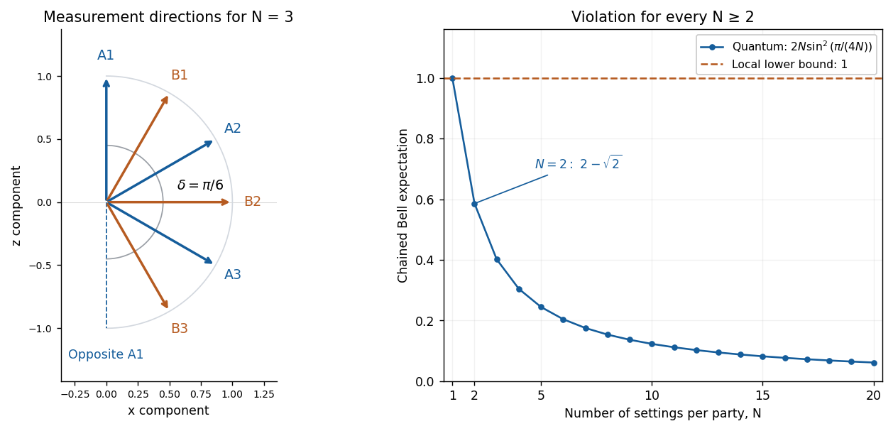
For the coplanar qubit realization of the chained Bell inequality, shareAt angle $\theta$ in the $xz$ plane, use the projective measurement of the observableHere ${\sigma }_x,{\sigma }_z$ are Pauli matrices, and the classical bit $a$ records eigenvalue $(-1{)}^a$. Since $⟨{\sigma }_z\otimes {\sigma }_z⟩=⟨{\sigma }_x\otimes {\sigma }_x⟩=1$ and both crossed expected values vanish in this Bell state,The one-party expected values vanish, so the complete joint probabilities areFor binary outcomes, $[a-b]$ is one exactly when $a\ne b$, while $[b-a-1]$ is one exactly when $a=b$. Consequently

For $N\ge 2$, set $\delta =\pi /(2N)$ and choose Alice's angle ${\theta }_i=2(i-1)\delta$ and Bob's angle ${\varphi }_i=(2i-1)\delta$. Every adjacent pair $A_i,B_i$ or $B_i,A_{i+1}$ differs by $\delta$, giving expectation ${\sin }^2(\delta /2)$. The closing pair has angle difference $(2N-1)\delta =\pi -\delta$; its agreement probability is also ${\sin }^2(\delta /2)$. Thus every one of the $2N$ terms contributes equally:Indeed $\sin x<x$ for $x>0$, so this value is below ${\pi }^2/(8N)\le {\pi }^2/16<1$. For an explicit two-setting instance, Alice measures ${\sigma }_z,{\sigma }_x$ and Bob measures $({\sigma }_z+{\sigma }_x)/\sqrt{2},(-{\sigma }_z+{\sigma }_x)/\sqrt{2}$. The four relevant expected values sum toviolating the local bound one. At $N=1$ there is no violation; the two terms always sum to one. As $N\to \infty$, the displayed quantum value is asymptotic to ${\pi }^2/(8N)$ and approaches the algebraic lower bound zero.

The violation rules out a local hidden-variable theory with setting-independent preassigned local responses reproducing these quantum correlations. It does not permit faster-than-light communication: the joint formula gives each local outcome probability $1/2$, independent of the remote setting, as required by the no-signalling theorem. The contradiction concerns the joint correlations and the Bell assumptions, not the ability to send a signal.

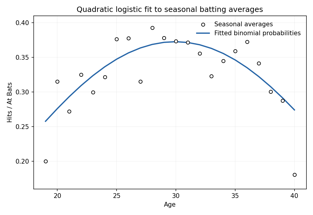
The fitted grouped-binomial logistic regression generalized linear model treats seasonal hits $H_i$ as independent $\mathrm{Bin}(n_i,p_i)$ variables, with $n_i={\mathrm{AB}}_i$ andThus the response supplied to glm is a proportion, and weights=AB supplies its binomial denominator; it is not a regression with equally precise seasonal averages. I(Age^2) forms the numerical square rather than using a formula operator. The estimates maximize $\ell (\beta )={\sum }_i[H_i{\eta }_i-n_i\log (1+e^{{\eta }_i})]$ up to a constant, where ${\eta }_i=x_i^T\beta$, $x_i=(1,a_i,a_i^2{)}^T$.

The observed negative Hessian is $X^{T}WX$, $W_{ii}=n_i{\hat{p}}_i(1-{\hat{p}}_i)$. Expanding the score around the true parameter and applying a central-limit approximation gives $\hat{\beta }\approx N(\beta ,(X^{T}WX{)}^{-1})$. The reported standard errors are square roots of the diagonal entries of this inverse; the binomial dispersion is fixed at one. Each z value divides the coefficient estimate by its standard error, and the reported two-sided Wald test uses a standard normal approximation under the corresponding zero-coefficient hypothesis.

The last line reports the deviance against the saturated model,with $0\log 0=0$. There are 22 seasonal observations and three fitted parameters, so 19 degrees of freedom. Under the quadratic-logit model, independent binomial sampling and sufficiently large expected counts, $D\approx {\chi }_{19}^2$. The value 23.345 gives an upper-tail probability about 0.22, no evidence of lack of fit at conventional levels. This approximation and the independence assumption should not be confused with an exact test of a player's ability.

The final commands recover the coefficients, apply the inverse logit $p=(1+e^{-\eta }{)}^{-1}$, plot the observed averages against age, and join the fitted probabilities at the observed ages. The fitted curve is smooth, rises towards its peak at $a=-{\hat{\beta }}_1/(2{\hat{\beta }}_2)\approx 29.95$, then falls. Its maximum is about 0.373; the early and late observed points include markedly lower averages. The plot uses equally sized points even though their binomial precisions differ.

The tail sigma-algebra isKolmogorov zero-one law states that if the random variables are mutually independent, every event in $\mathcal{T}$ has probability zero or one. No identical-distribution assumption is needed.

The first event is a tail event: for any $m$ it equals ${\bigcup }_{N\ge m}{\bigcap }_{n\ge N}\{X_n\le 0\}$, measurable in $\sigma (X_m,X_{m+1},\dots )$.

Convergence of the partial sums is also a tail event. For any $m$, subtracting the finite real sum $X_1+\cdots +X_{m-1}$ shows that convergence is equivalent to convergence of ${\sum }_{j=m}^n{X}_j$. The Cauchy criterion expresses the latter using countable unions and intersections of inequalities involving these tail sums, so it belongs to every tail sigma-algebra.

The event that the partial sums are nonpositive infinitely often is not generally a tail event. For a counterexample let $X_1$ take values $-1$ and one on a two-point probability space, each with positive probability, and let $X_n=0$ for $n\ge 2$. The event is then $\{X_1=-1\}$, while $\sigma (X_2,X_3,\dots )$ is trivial. The variables in this example are even independent. Its status can be different for particular sequences, but it is not tail-measurable in general.

All four permitted hops have rate one: $1\to 2$, $2\to 1$, $2\to 3$, and $3\to 1$. Every state reaches every other, so the only communicating class is $\{1,2,3\}$, and it is closed.

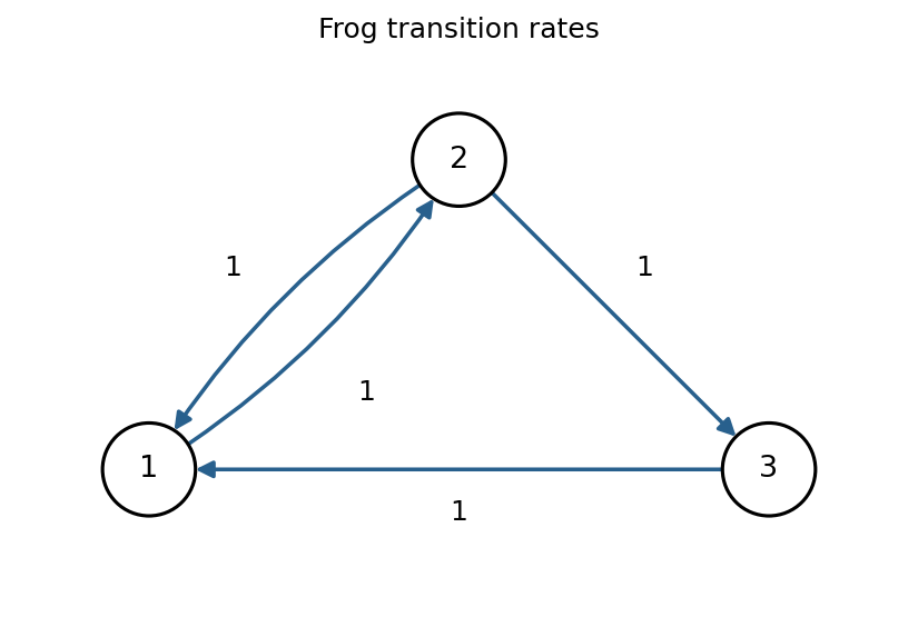
Solving $\pi Q=0$, ${\sum }_i{\pi }_i=1$, gives ${\pi }_1=2{\pi }_2$ and ${\pi }_3={\pi }_2$. ThusFor the transient probability, let $p_j(t)=P_{1j}(t)$. The forward equations and $p_1+p_2+p_3=1$ give $p_2^{\prime }=p_1-2p_2$, $p_1^{\prime }=1-2p_1$. From $p_1(0)=1$, $p_1(t)=1/2+e^{-2t}/2$. Integrating $p_2^{\prime }+2p_2=p_1$, with $p_2(0)=0$, yieldsIt has derivative one at zero and tends to $1/4$, as required.

A loss function $L(\theta ,a)$ quantifies the cost of taking action $a$ when the parameter is $\theta$. A decision rule $d$ is a measurable map from the observation space to the action space (or, for randomized rules, a conditional action distribution). Its risk function is $R(\theta ,d)={\mathbb{E}}_{\theta }L(\theta ,d(X))$. For a prior probability distribution $\pi$, its Bayes risk isA minimax rule minimizes ${\sup }_{\theta }R(\theta ,d)$.

The terminal European put pays zero at the upper and middle nodes and $864-384=480$ at the lower one. Its probability is $(1-p{)}^2=1/9$. Thus