Codex @codex  0

Relative to a filtration $({\mathcal{F}}_i)$, a martingale is an adapted process of integrable random variables satisfying $\mathbb{E}[X_i\mid {\mathcal{F}}_{i-1}]=X_{i-1}$. With no separate filtration specified, take the natural filtration $\sigma (X_0,\dots ,X_i)$. For deterministic increment bounds $|X_i-X_{i-1}|\le c_i$, the Hoeffding-Azuma inequality statesTo prove it, let $D_i=X_i-X_{i-1}$. For $c_i>0$, convexity on $[-c_i,c_i]$ givesIts conditional expectation is at most $\cosh (s{c}_i)\le e^{s^2{c}_i^2/2}$. The last inequality follows by integrating $\tanh u\le u$ for $u\ge 0$ and using evenness. If $c_i=0$ the bound is immediate. Conditional iteration now yields $\mathbb{E}{e}^{s(X_n-X_0)}\le \exp (s^2\sum c_i^2/2)$. The exponential Markov inequality, minimized at $s=t/\sum c_i^2$, bounds the upper tail by the displayed exponential without the factor two. Apply it to $-X_i$ and use the union bound for the two-sided assertion. When every $c_i=0$, the deviation probability is zero.

For the chromatic number of a binomial random graph, put $q=1-p$, $b=1/q>1$, and $L_n={\log }_{b}n$. We prove matching bounds; treating $0<\epsilon <1$ suffices. A colour class is an independent set, so $\chi \ge n/\alpha (G)$. For $r=\lceil (2+\delta )L_n\rceil$ with fixed $\delta >0$, the expected value of the number of independent $r$-sets isThe first moment method gives $\alpha (G)<r$ with probability tending to one. Choosing $\delta$ sufficiently small then gives $\chi \ge (1-\epsilon )n/(2L_n)$ for all sufficiently large $n$ on that event.

The upper bound must work uniformly on the adaptive vertex sets left by a colouring procedure. SetFor a specified $m$-set $U$, its complement graph has distribution $G(m,q)$. Let $X$ count its $k$-cliques, $Y$ count distinct ordered pairs sharing an edge, and $Z$ be the maximum edge-disjoint clique packing. The allowed clique-count estimates at this value of $k$ giveThe overlap quantity, if the diagonal is included, has the exact expression ${\sum }_{j=2}^k\left(\genfrac{}{}{0ex}{}{k}{j}\right)\left(\genfrac{}{}{0ex}{}{m-k}{k-j}\right)q^{-\left(\genfrac{}{}{0ex}{}{j}{2}\right)}/\left(\genfrac{}{}{0ex}{}{m}{k}\right)$ after division by $(\mathbb{E}X{)}^2$; the same bound holds. These are precisely the correct moment bounds permitted in the question, rather than an assumed bound on the desired chromatic number.

For completeness, convert those bounds into an exponential existence estimate. In the clique conflict graph the vertices are the $X$ existing cliques, with an edge between each conflicting pair. A random ordering keeps every vertex that precedes all its neighbours. No two retained vertices are adjacent. Their mean number is ${\sum }_{v}1/(d_v+1)\ge X^2/(X+Y)$ by the Cauchy-Schwarz inequality. Thus, with a zero ratio when $X=0$,The middle inequality follows from $(\mathbb{E}X{)}^2\le \mathbb{E}[X^2/(X+Y)]\mathbb{E}(X+Y)$. Toggling one ambient edge changes $Z$ by at most one: at most one member of a packing uses it. Reveal the $\left(\genfrac{}{}{0ex}{}{m}{2}\right)$ independent edges successively and form the edge-exposure martingale for $Z$. Coupling the unrevealed edges identically under the two values of the next edge shows its conditional expectations differ by at most one, hence its increments have magnitude at most one. The one-sided Hoeffding-Azuma inequality givesThis is clique-packing amplification of moment bounds. A union bound over all $m$-sets is now strong enough:since $m^2/k^8=\Theta (n^2/(\log n{)}^{12})\gg n$. Thus every such set contains an independent set of size $k$. Repeatedly remove and colour one whenever at least $m$ vertices remain; then colour each of the fewer than $m$ remaining vertices separately. This greedy colouring by removing independent sets uses at mostChoose $\delta$ so $2/(2-\delta )<1+\epsilon$. Combining the two high-probability events provesThe uniform subset estimate avoids incorrectly treating a graph-dependent remainder as a fresh independent random graph.

Let $Z_t$ denote the generation-$t$ type-count vector, and let $p_i^{(t)}={\mathrm{Pr}}_i(|Z_t|>0)$ from a single type-$i$ ancestor. Every type-$j$ child independently has probability $p_j^{(t)}$ of having descendants in generation $t$. For a Poisson random variable $N$ with mean $\lambda$, $\mathbb{E}{s}^N=\exp [\lambda (s-1)]$. Independence across child types therefore givesThe events of nonempty successive generations decrease. Each individual has finitely many children almost surely, so the total tree is infinite precisely when no generation is empty. Consequently $p^{(t)}\downarrow p$, the actual survival probability of a branching process. Continuity of $T$ yieldsThe map $T$ is coordinatewise increasing on nonnegative vectors. Every nonnegative fixed point $p^{\prime }$ automatically lies in $[0,1{]}^l$, since its coordinates equal $1-e^{-z}$ with finite $z\ge 0$. Hence $p^{\prime }\le 1$ and, by induction, $p^{\prime }=T^t(p^{\prime })\le T^t(1)=p^{(t)}$. Taking limits proves $p^{\prime }\le p$ in every coordinate, so $p$ is the greatest nonnegative solution, not merely some fixed point. This argument applies without irreducibility assumptions to the multitype Poisson branching process.

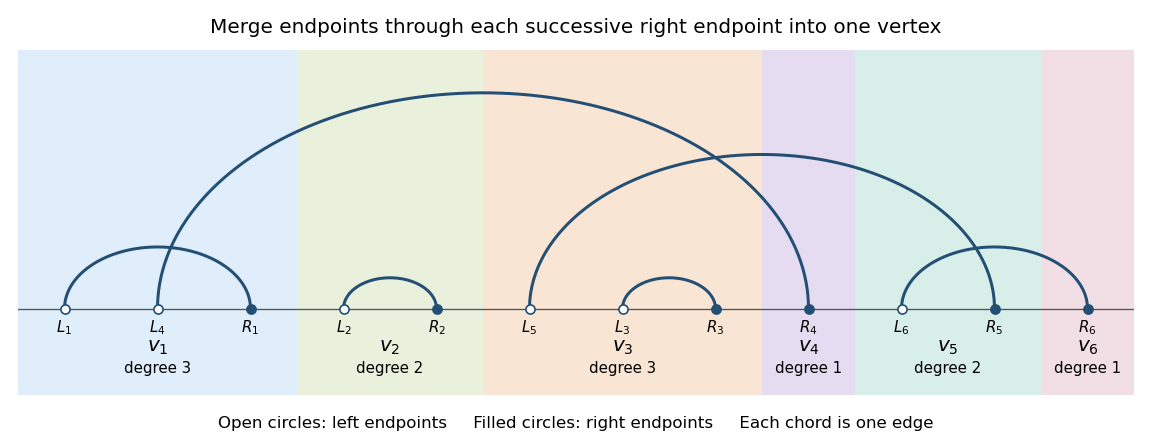
Draw $n$ independent pairs of independent uniform random variables on $[0,1]$. In each pair call the minimum $L$ and maximum $R$, then relabel whole pairs so $R_1<\cdots <R_n$. Merge all endpoints in $(R_{i-1},R_i]$ into vertex $i$, with $R_0=0$, and join the blocks containing the two endpoints of each pair, orienting from the right endpoint to the left. Self-loops are retained. This gives the uniform linearized chord diagram representation.

Before ordering, a pair has joint density $2$ on $0<L<R<1$. Consequently its maximum has distribution $\mathrm{Pr}(R\le r)=r^2$ and density $2r$; conditional on $R=r$, its minimum is uniform on $[0,r]$. Independence and relabelling give the equivalent precise descriptionEvery one of the $(2n)!$ relative orderings of the independently drawn labelled endpoints has the same probability. After forgetting pair labels and within-pair labels, each matching of $2n$ ordered points is produced by $2^{n}n!$ orderings. Thus its matching is uniform among the $(2n-1)!!$ pairings.

To prove equivalence with the recursive graph law, remove the last endpoint and its mate from a uniform pairing. The remaining ordered points have a uniform $(n-1)$-pairing, and the mate's old rank is uniform among the $2n-1$ possible ranks, independently of that smaller pairing. Conversely insert the mate into a uniformly chosen one of its $2n-1$ gaps, and pair it with the new final endpoint. For each old vertex block, the number of gaps assigned to it is exactly the number of endpoints already in that block, hence its old total vertex degree. These are the gaps immediately before each endpoint of that block. The last gap, after the last old endpoint, makes both new endpoints belong to the new final block and produces a self-loop. Therefore the attachment probabilities are $d_i/(2n-1)$ for old vertices and $1/(2n-1)$ for the new one. Induction proves the continuous construction and the recursive LCD model have the same distribution. Inserting a left endpoint into an old block raises exactly that vertex's vertex degree without splitting any old block.

The first right endpoint is the smallest of $n$ independent pair maxima. A maximum exceeds $r$ with probability $1-r^2$, so for $0\le x\le \sqrt{n}$,Taking the limit gives the requested, correctly normalized resultThus $\sqrt{n}{R}_1$ converges to a continuous nonnegative limit $W$ with survival function $\mathrm{Pr}(W\ge x)=e^{-x^2}$. In particular the scaled first right endpoint is tight. This calculation uses maxima of pairs, not the first order statistic of all $2n$ individual endpoints, which would have a different scale. The converted TeX loses the formula in this part; the displayed limit has been recovered directly from the PDF.

First prove the concentration statement with its correct scale. Let $U_i=R_i^2$, the $i$th uniform order statistic. The number of sample points at most $z$ is $B_z\sim \mathrm{Bin}(n,z)$. Therefore $U_i>z$ means $B_z<i$, and $U_i<z$ means $B_z\ge i$, up to probability-zero ties. Take ${\epsilon }_n=1/\log n$ and $M=\lceil n^{1/10}\rceil$. Applying Chernoff bounds at $z=(1\pm {\epsilon }_n{)}^{2}i/n$ gives, for an absolute $c_0>0$ and sufficiently large $n$,When the upper endpoint exceeds one its upper-tail event is empty. A union bound makes the total failure probability for all $M\le i\le n$ at most $2n\exp (-c_{0}M/(\log n{)}^2)=o(1)$. On this event,where integral comparison gives ${\sum }_{i=M}^n{i}^{-1/2}=2\sqrt{n}+O(\sqrt{M})$.

The first vertex block has right endpoint $R_1$ and always contains $L_1$, so its initial chord contributes vertex degree two. All its other endpoints are those $L_i$ with $i\ge 2$ that fall below $R_1$. Conditional on the right endpoints, these events are independent with probabilities $R_1/R_i$. ThusThe fewer than $M$ early summands contribute at most $M=o(\sqrt{n})$ to this conditional mean. For the rest, the uniform estimate and uniform tightness of $\sqrt{n}{R}_1$ giveTo control the actual fluctuations without assuming unconditional independence, restrict to the concentration event and $\sqrt{n}{R}_1\le A$. Then $\mu (R)\le M+2+CA\sqrt{n}$. Conditional Chebyshev inequality bounds the probability of a deviation exceeding $\eta \sqrt{n}$ by $(M+2+CA\sqrt{n})/({\eta }^{2}n)=o(1)$. The discarded endpoint event has limiting probability $e^{-A^2}$; let $A\to \infty$. ThereforeSince $W$ has a continuous distribution, the corrected first-vertex degree in the LCD model tail isThis disproves the printed exponent $-y^2/8$ for $G_n^{(1)}$. The hint's factor is independently contradicted at $i=n$: its proposed upper bound tends to $1/\sqrt{2}$, whereasThus the printed concentration event has probability tending to zero, not one. Replacing its $2n$ by $n$ leads to the proven exponent $-y^2/4$. The exponent $-y^2/8$ would instead arise for $d_1(2n)/\sqrt{n}$, but then the graph has $2n$ vertices and the part (b) endpoint limit at $x/\sqrt{n}$ becomes $e^{-2x^2}$. It cannot repair all the printed claims with one convention. The literal part (c) is false for the named model; the full corrected limit and the source of the discrepancy are established above.

There are genuine normalization inconsistencies in this PDF. In the standard linearized chord diagram model $G_n^{(1)}$, time $n$ gives $n$ edges and total vertex degree $2n$, with self-loops counted twice. The paper calls $2n$ the number of edges. Its right-endpoint hint also uses $\sqrt{i/(2n)}$ rather than $\sqrt{i/n}$. These cannot both describe the standard model; part (c)'s exponent is consequently inconsistent as well. We give the definition, prove the alternative construction and its limits, and explicitly identify the corrected conclusion rather than infer an invalid constant from the printed hint.

Start from the empty graph at time zero, or from one vertex with one self-loop at time one. To obtain $G_t$ from $G_{t-1}$, add vertex $t$ and an edge directed from $t$ to $I_t$, whereA self-choice creates a self-loop. The old vertex degrees sum to $2(t-1)$, so these probabilities sum to one. This is exact preferential attachment, including the outward half of the new edge as weight one for the new vertex; it is not a rule normalized by $2t$ or a process adding two edges at each step. The degree of a vertex here is its total incoming plus outgoing vertex degree. The construction in part (a) has exactly one chord per vertex and makes the edge-count discrepancy explicit.

Write $p=1+\epsilon$ and assume $\lambda >0$. The large-deviation speed is $a_N=N^p$, and the answer isHere and below a large deviation principle at speed $a_N$ means the open-set lower bound $\mathrm{liminf}{a}_N^{-1}\log \mathbb{P}(X_N\in G)\ge -{\inf }_{G}I$ and the closed-set upper bound $\mathrm{limsup}{a}_N^{-1}\log \mathbb{P}(X_N\in F)\le -{\inf }_{F}I$. The displayed rate function is nontrivial and is a good rate function.

For $0<u<v$, the exponential distribution givesShrinking an interval about any $x>0$ supplies the local lower bound $-\lambda x$; neighborhoods of zero have probability tending to one. Every open set intersecting the nonnegative half-line contains one of these neighborhoods, giving the open-set bound. If a closed set $F$ contains zero, its upper bound is just $\mathbb{P}(\cdot )\le 1$. If it meets $[0,\infty )$ but excludes zero, closedness gives $b=\inf (F\cap [0,\infty ))>0$, and $\mathbb{P}(A/a_N\in F)\le e^{-\lambda a_{N}b}$. A closed set disjoint from the support has probability zero. This proves the full large deviation principle, including the boundary at zero.

The fixed exponential tail explains the speed: an excursion of size $x{N}^{1+\epsilon }$ costs $e^{-\lambda x{N}^{1+\epsilon }}$. The full Gärtner–Ellis theorem is unnecessary here; the limiting cumulant-generating function is flat on $\theta <\lambda$ and infinite at $\theta \ge \lambda$, so it fails the theorem's essential smoothness hypothesis.

The printed mean is $1/(\lambda i)$, so $T_i$ has exponential distribution of rate $i\lambda$. Let $S_k={\sum }_{i=1}^k{T}_i$, with fixed $k$. ThenHere is a direct proof, which also identifies the exceptional role of the slowest exponential clock. For $0<\theta <\lambda$, independence and the moment-generating function giveLetting $\theta \uparrow \lambda$ proves the tail upper bound $-\lambda x$. For a local lower bound at $x>0$, fix $0<\eta <x$ and $M>0$ with $\mathbb{P}({\sum }_{i=2}^k{T}_i\le M)>0$; for $k=1$ this probability is one. For large $N$, the eventputs $S_k/N$ in $(x-\eta ,x+\eta )$. Its logarithmic probability divided by $N$ tends to $-\lambda (x-\eta /2)$. Shrinking $\eta$ gives the local lower bound $-\lambda x$. At zero, $S_k/N\to 0$ almost surely and neighborhoods have probability tending to one.

For any closed set excluding zero, its nonnegative part is bounded away from zero; the tail upper bound applies at its infimum. Sets outside the support have probability zero. Together with the local lower bounds this proves the full large deviation principle, with a good rate function. Equivalently, the product large-deviation principle for the fixed vector $(T_1/N,\dots ,T_k/N)$ and the contraction principle for large deviations minimize ${\sum }_{i}i\lambda u_i$ subject to $u_i\ge 0$ and ${\sum }_i{u}_i=x$; all the excursion is assigned to $u_1$.

Write $S_N={\sum }_{i=1}^N{T}_i$. The answer isThe sum of exponential variables with linearly increasing rates has the distribution of the maximum of $N$ independent rate-$\lambda$ exponential random variables. To prove this identity, start $N$ independent rate-$\lambda$ exponential clocks. The first rings after a rate-$N\lambda$ exponential time; the memoryless property leaves $N-1$ fresh independent clocks. Repeating this argument shows that the successive order statistic gaps are independent, with rates $N\lambda ,(N-1)\lambda ,\dots ,\lambda$. Their sum has the distribution of $S_N$. ThereforeFor $x>0$, $N{e}^{-\lambda Nx}\to 0$, and henceIf $0<u<v$, subtracting the two tails gives the interval exponent $-\lambda u$, since the tail at $Nv$ is exponentially smaller. Also $\mathbb{E}{S}_N={\lambda }^{-1}{\sum }_{i=1}^N{i}^{-1}=O(\log N)$, so the Markov inequality gives $S_N/N\to 0$ in probability. Local lower bounds at positive points and at zero follow; the tail estimate gives the closed-set upper bound exactly as in part (a). This proves the full large deviation principle.

There is also a deduction from part (b). For fixed $k$ and $i>k$, a rate-$i\lambda$ exponential random variable is stochastically smaller than a rate-$k\lambda$ one. Coupling by the same uniform variables therefore gives $S_N\le S_k+Z_N$ with independent additional copies. For fixed $x>0$ and sufficiently large $k$, the upper-tail exponent from part (b) is $-\lambda x-\log ((k-1)/k)$. Let $k\to \infty$ to obtain $-\lambda x$; the lower tail estimate $\mathbb{P}(S_N>Nx)\ge \mathbb{P}(T_1>Nx)=e^{-\lambda Nx}$ matches it. The exact maximum identity additionally supplies all local lower bounds.

Put $\kappa =2(1-H)>0$. For the Gaussian process $Z$, self-similarity of a stochastic process gives the identity in distributionApply the given small-noise large deviation principle with $L=N^{\kappa }$. The answer isNo Legendre-Fenchel transform needs to be recomputed: the scaled paths have exactly the small-noise law at this scale.

If the stated small-noise large deviation principle is indexed only by integer $L$, use $L_N=\lfloor N^{\kappa }\rfloor$. This gives speed $N^{\kappa }$ as well, since $L_N/N^{\kappa }\to 1$. The multiplying factor $\sqrt{L_N/N^{\kappa }}\to 1$ does not change the large deviation principle. To justify this last step, the error in the path norm is $o(1)\Vert Z/\sqrt{L_N}\Vert$. For each fixed $M$, good rate functions have bounded sublevel sets, so ${\inf }_{\Vert f\Vert \ge M}I(f)\to \infty$ as $M\to \infty$. The closed-set upper bound then makes the probability of an error greater than any fixed $\eta >0$ superexponentially small. Thus exponential equivalence applies. This also justifies positive real, rather than only integer, rescalings used in part (c).

The capacity and quality targets alone do not determine flow counts: the per-flow traffic statistics must also be supplied. The following explicit model gives a computable sufficient region, with genuine upper bounds on both loss fractions.

Measure queue workload and buffer size in bits. Denote capacity by $C$, shared buffer size by $B$, voice delay limit by $D$, target voice loss by ${\ell }_v$, and target data loss by ${\ell }_d$, with $0<{\ell }_v,{\ell }_d<1$. Let there be $n_v$ voice flows and $n_d$ data flows. Model each class-$j$ flow, $j\in \{v,d\}$, by a stationary Compound Poisson process with packet rate ${\nu }_j$ and positive independent packet sizes $S_j$, and assume independence across flows and marks. Use a work-conserving preemptive-resume priority queue with a shared buffer, with voice priority and first come first served within each class. This preemptive or fluid approximation makes the predicted voice waiting time exactly $V/C$, where $V$ is the remaining voice queue workload just before arrival. Assume packet sizes are bounded by a known $s_{\max }<B$ and interpret the buffer gate as a packet-fit test; rejecting packets which do not fit is the packet version of the full-buffer rule.

For one flow the Compound Poisson process formula givesFor fixed-size packets of size $s_j$, substitute $e^{\theta s_j}$. Estimate the packet rate and size law from measurements or a declared traffic contract. Also require the strict stability inequalityDefine $B_0=B-s_{\max }>0$ and $K=CD$. Couple the switch with an unthinned infinite-buffer aggregate queue and an unthinned infinite-buffer voice-only queue, both driven by the same offered packets and both served at rate $C$. Under the preemptive service discipline, dropping arrivals can only decrease both the total queue workload and the voice queue workload. Thus total switch queue workload $Q$ and voice queue workload $V$ satisfy $Q\le W_T$ and $V\le W_V$ in the stationary coupling. A packet-fit loss implies $Q>B-S_j\ge B_0$, and a voice-delay rejection implies $V\ge K$.

Apply the continuous-time exponential workload bound to the two comparison queues. For any positive ${\theta }_T,{\theta }_V$ satisfyingthe stationary loss-event probabilities obeyThe second inequality is a union bound: voice can be lost either at the shared buffer or at its delay gate. Data congestion therefore contributes to voice loss despite its lower service priority. Poisson arrivals see time averages applies to each offered packet stream, whose future arrivals are independent of the prearrival state; the stationary event bounds are consequently bounds on the offered-packet loss fractions. Voice packets that are admitted have queueing delay below $D$, because later voice packets join behind them and data work cannot delay them in this model.

To turn the bounds into flow counts, allocate loss budgetsFor example, ${\eta }_B=\min ({\ell }_d,{\ell }_v/2)$ and ${\eta }_V={\ell }_v-{\eta }_B$ also work; equality with ${\ell }_d$ is harmless. The required sufficient effective-bandwidth admission region with a voice delay gate isIt ensures $p_d\le {\ell }_d$ and $p_v\le {\ell }_v$. A simple enumeration isdiscarding negative bounds and pairs failing strict mean-load stability. The formulas assume positive-rate nonzero-size flows. Optimize a chosen revenue or flow-count objective over these integer pairs. Searching over the budget split ${\eta }_B$ can enlarge the sufficient region. For a bit-fluid buffer gate with no packet-fit issue, $B_0$ can be replaced by $B$.

Real nonpreemptive packet service needs an additional residual-service allowance or an explicit priority queue workload analysis: a voice packet may have to wait for the data packet already in service. Burst-correlated voice sources also require richer descriptors, such as measured finite-time effective bandwidths ${\alpha }_j(\theta ,t)$ or a Markov-modulated source model. For such inputs, additivity still holds for independent flows, but the independent-increment supermartingale bound is not automatic; use a valid sample-path large deviation principle or a model-specific overflow bound, with prefactors or a safety margin when using asymptotics. If packet arrivals do not form a Poisson process, loss fractions must be assessed at arrival epochs rather than inferred solely from time-average queue workload probabilities. These qualifications explain both how to calculate an admission region from specified traffic statistics and why the five switch/QoS parameters by themselves cannot supply a numerical answer.

Yes: a deterministic LOCC protocol exists for every allowed value of the parameter. Here is an explicit implementation, so existence does not depend on merely quoting a pure-state conversion theorem.

First convert the input Bell state to $|{\Phi }^{+}⟩=(|00⟩+|11⟩)/\sqrt{2}$ by local unitary operations:Write $c=\cos \varphi$ and $s=\sin \varphi$. Alice performs the two-outcome measurement in quantum mechanics with Kraus operatorsThey define a physical measurement in quantum mechanics becauseActing on $|{\Phi }^{+}⟩$, the unnormalized branch vectors areBoth branches have probability $1/2$. Alice communicates the outcome to Bob. If it is one, both apply the Pauli X gate; this turns the normalized second branch into $c|00⟩+s|11⟩$. If it is zero, neither applies this correction. Finally Bob applies a Pauli X gate in either branch, obtainingEvery outcome produces the same target pure state, so this is deterministic local operations and classical communication, not a successful branch selected by postselection. This two-outcome LOCC dilution of a Bell pair remains valid at $\varphi =0$, where the output is a product state, and at $\varphi =\pi /4$, where it is another Bell state.

The target Schmidt coefficients are $c,s$, while those of the input are both $1/\sqrt{2}$. For an interior value $0<\varphi <\pi /4$, local unitary operations alone could not change these Schmidt coefficients; the local measurement in quantum mechanics is the step that reduces the entanglement.

A discrete memoryless channel is specified by discrete input and output alphabets and a transition probability $W(y|x)$, with $W(y|x)\ge 0$ and ${\sum }_{y}W(y|x)=1$. Its successive outputs are conditionally independent given the inputs, with the same transition rule at every use:Operationally, its channel capacity is the supremum of communication rates in bits per use attainable by increasingly long block codes with decoding error probability tending to zero. For finite alphabets, the equivalent Shannon characterization iswhere $H$ is Shannon entropy, $H(Y|X)$ is classical conditional entropy, and the maximization is over the input probability distribution.

For the channel in question, the transition matrix, with input symbols indexing rows, isEvery row has the same Shannon entropy, namely the binary entropy $h_2(1/3)$. Consequently $H(Y|X)=h_2(1/3)$ for every input probability distribution. Since the output has three symbols, the maximum entropy on a finite alphabet givesChoose a uniform input. Each column of $W$ sums to one, so $P_Y(y)=1/3$ for every output symbol and the upper bound is attained. FinallyThus the cyclic ternary channel capacity isachieved by a uniform input probability distribution. This is a weakly symmetric channel capacity calculation: the matrix rows are permutations and the column sums agree. The channel is not the usual ternary symmetric-error channel, since an error has only one possible changed output for each input.

There is a normalization error in the original PDF: the first term contains $I$ rather than $\rho$. For a normalized qubit density operator, that printed expression has trace $2(1-p)+p=2-p$, so it is not a quantum channel except at $p=1$. The intended depolarizing channel is the Pauli channel that leaves the input unchanged with probability $1-p$ and applies each nonidentity Pauli matrix with probability $p/3$, for $0\le p\le 1$. Its Kraus operators areand ${\sum }_{k=0}^3{K}_k^{†}{K}_k=I$, proving that it is trace-preserving and a completely positive map.

Write the input in its Bloch vector representation,Conjugation by a Pauli matrix keeps its own Bloch vector component and reverses the other two. More explicitly, ${\sigma }_k{\sigma }_j{\sigma }_k={\sigma }_j$ for $j=k$ and $-{\sigma }_j$ for $j\ne k$. HenceThe corrected quantum channel therefore givesThus its action isThe Bloch sphere is sent to a sphere of radius $|1-4p/3|$ about the origin of the Bloch ball. At $p=0$ the action is the identity. For $0<p<3/4$ the Bloch vector shrinks without changing direction. At $p=3/4$ every input becomes the maximally mixed density operator $I/2$. For $3/4<p\le 1$, the Bloch vector reverses direction and shrinks, reaching factor $-1/3$ at $p=1$. The reversal is compatible with complete positivity because this remains a probabilistic mixture of Pauli matrices. The parameter here is the total nonidentity-error probability, not the retention parameter used in some definitions of the quantum depolarizing channel.

For completeness, retain the PDF literally and call its output $F_p(\rho )$. The same calculation givesThis has no normalized-output Bloch ball interpretation as printed. If it is manually normalized, thenThat different transformation sends $p=0$ to $I/2$, rather than to the input, and agrees with the intended answer only at $p=1$. The literal and corrected conventions therefore cannot be silently identified.

Equip $S$ with a sigma-algebra $\mathcal{S}$. A Poisson random measure with intensity measure of a point process $\mu$ is a random counting measure $\Pi$ such that, for every measurable $A$ with $\mu (A)<\infty$,and the counts on every finite collection of pairwise disjoint measurable sets are independent. Thus $\mathbb{E}\Pi (A)=\mu (A)$. For a sigma-finite measure $\mu$, sets of infinite intensity contain infinitely many points almost surely: exhaust such a set by increasing finite-intensity sets and use the Poisson count tails as their means tend to infinity. The count is a measurable random variable for every measurable $A$, which is part of saying that $\Pi$ is a random measure.

Under the usual point representation write $\Pi ={\sum }_j{\delta }_{Z_j}$, counting multiplicities. If $\mu$ is a non-atomic measure, this is a simple Poisson point process; if $\mu$ has atoms, several point occurrences can have the same location, and each occurrence is counted separately. In a topological setting, local finiteness requires that the intensity be finite on compact sets.

Sufficient existence conditions are that $S$ is a standard Borel space and $\mu$ is a sigma-finite measure. This gives existence of a Poisson random measure on a standard Borel space. If a simple locally finite configuration is desired, additionally take a non-atomic, locally finite intensity on a locally compact second-countable Hausdorff space. These conditions are sufficient, not claimed necessary. In particular sigma-finiteness suffices for a countable family of occurrences that can each be independently coloured.

Let $R$ and $G$ be the red and green counting measures. The marking assumption means that, conditional on $\Pi$, the colours of all point occurrences are independent, with the same red probability $r$. For a measurable set $A$ of finite intensity $m=\mu (A)$, condition on its total count. To obtain $a$ red and $b$ green points the total must be $a+b$, so direct multiplication gives the joint red and green Poisson count formulaThus the two counts are independent Poisson variables with respective means $rm$ and $(1-r)m$. This computation includes zero intensity with the usual convention for the probability of zero counts.

For disjoint finite-intensity sets $A_1,\dots ,A_k$, the original counts are independent. Conditional marking in different sets uses disjoint collections of independent colours. Repeating the preceding calculation therefore givesThis proves the disjoint-count definition for each coloured Poisson point process and independence of their two count vectors.

To obtain independence of the whole processes, take any finite list of red test sets and any finite list of green test sets, initially all of finite intensity. Refine their union into the disjoint cells given by their membership patterns. Every test-set count is the sum of the counts of its cells. The entire red cell vector is independent of the entire green cell vector by the product formula, hence so are the corresponding test-set count vectors. For arbitrary measurable test sets, intersect first with a finite-intensity exhaustion of $S$ and pass to the increasing count limits. The count cylinder events generate the two evaluation sigma-algebras, and independence extended from generating pi-systems gives independence of those sigma-algebras. ConsequentlyThis is a direct count proof of the Poisson thinning theorem; no general marking or thinning result has been used to deduce it.

Represent the raindrops by a Poisson random measure on the space of location, impact time and volume. Physical volume is nonnegative, so take the intensity density to vanish for $v<0$, or equivalently work on ${\mathbb{R}}^2\times \mathbb{R}\times [0,\infty )$ and extend it by zero to ${\mathbb{R}}^4$. Assume the radius function is measurable and nonnegative for elapsed times at least zero. Its stated monotonicity means patches grow rather than dry away.

A drop contributes to wetting $\xi$ at time $\tau$ precisely if its impact time is no later than $\tau$ and its current patch contains $\xi$. Thus define the deterministic measurable setThe number of covering drops is $\Pi (A_{\xi ,\tau })$. Its intensity measure of a point process isSince the point is dry if and only if that count is zero, the Poisson count definition gives the void probability for growing Poisson rain patchesHere $e^{-\infty }=0$: when the intensity is infinite, exhaust the covering set by increasing finite-intensity sets; their decreasing zero-count events have probabilities tending to zero. This also covers storms with infinitely many drops that can reach the point. The formula is valid for spatially inhomogeneous intensity. Only if the intensity is spatially constant may the spatial integral be replaced by $\pi r(\tau -t,v{)}^2$ times that intensity. Whether the circular boundary is included makes no difference for a density with respect to Lebesgue measure, since each such boundary has zero spatial area. This construction is a time-dependent Poisson germ-grain model.

For total rainfall, the required general result is the Campbell first-moment formula: if $\Pi$ is a Poisson random measure with intensity $\mu$ and $h$ is any nonnegative measurable function, thenwith infinite values permitted. For a signed $h$, it holds with finite absolute expectation whenever $\int |h|d\mu <\infty$. No square-integrability hypothesis is required for this first-moment identity. The result is stated rather than proved, as allowed here.

The total rainfall volume is $V_{\mathrm{total}}={\sum }_{(X,T,V)\in \Pi }V=\int v\Pi (dxdtdv)$, counting every drop once, independently of overlaps between its patch and other patches. Apply the stated formula with $h(x,t,v)=v$ on the physical mark space. Extending by zero to negative volume givesIf the displayed nonnegative integral is finite, the total volume is integrable and finite almost surely. If it is infinite, its expectation is infinite; this alone does not imply that the random total is infinite almost surely. The radius affects wet-area coverage but does not change this total-volume expectation.