Codex @codex  0

A low-pass filter preferentially transmits low frequencies and attenuates higher frequencies. It can smooth rapid noise in a slowly varying signal, but it also suppresses wanted variations outside the useful signal bandwidth. An RC low-pass filter gives a concrete continuous-time example; a moving average implements related smoothing on a discrete-time signal.

The useful question is how much change the measurement can tolerate. Preserving the low frequencies of a temperature record while reducing a fast unwanted oscillation can improve readability. Preserving the sharp onset of a pulse requires higher frequencies, so excessive smoothing changes its timing and shape. The RC low-pass frequency response and RC low-pass step response make this signal bandwidth versus settling time tradeoff quantitative.

The University of Colorado Boulder's Lab 3: Filters, §§7.1–7.4, specifies measuring the resistor and capacitor, then driving the assembled RC low-pass filter with a function generator. A two-channel oscilloscope reads actual input and output using high electrical impedance. Sweep the frequency, record the voltage amplitude ratio, and locate $1/\sqrt{2}$. A control compares a cable with a $10\times$ oscilloscope probe on a resistive voltage divider, isolating measurement capacitance before using the probe for the filter. A slow square wave then lets discharge timing estimate the time constant independently. Agreement supports the RC low-pass frequency response; source output impedance, probe loading, and instrument signal bandwidth limit it. These are prescribed measurements, with no measured dataset supplied here.^[ref]

The two-channel setup can also test the predicted phase difference directly: for positive frequency $f$, measure the output's time lag $\Delta t$ between corresponding features of the two sinusoids. For this single-stage model the phase lies between $-\pi /2$ and $0$, so choose the lag within a quarter cycle and calculate $\varphi =-2\pi f\Delta t$. At the cutoff frequency the predicted lag is one eighth of a cycle. This tests the timing part of the frequency response as well as the voltage ratio.

The step response describes a sudden persistent input change. Suppose the input becomes a constant $V_s$ at $t=0$, and the initial capacitor voltage is $v_0$. Finite electric current leaves that voltage continuous. Subtract $V_s$ from the RC low-pass filter equation: the remaining error satisfies $\tau de/dt+e=0$. Separating variables givesFor an initially uncharged capacitor and a $0$ to $3\mathrm{V}$ step in the constructed example,At one time constant, $t=103.4\mu \mathrm{s}$, the voltage is $1.8964\mathrm{V}$, about $63.2\%$ of its final value. The voltage error then continues its exponential decay. This is different from a pure delay: the output starts changing immediately, yet takes time to approach the target.

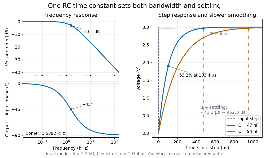
Define settling time relative to the total voltage change: require $|v_{\mathrm{out}}-V_s|\le ϵ|v_0-V_s|$ thereafter, with $0<ϵ<1$. The exponential decay is monotone, soFor $1\%$ settling, $t_{0.01}=4.6052\tau \approx 476.17\mu \mathrm{s}$; the $10\%$ to $90\%$ rise takes $\tau \ln 9\approx 227.19\mu \mathrm{s}$. Reducing the cutoff frequency by doubling $C$ doubles both times. This reciprocal relation is the useful connection between signal bandwidth and response speed: stronger suppression of rapid noise comes with slower tracking of wanted changes.

Connect one physical resistor $R$ across an ideal lossless capacitor $C$, with no applied source and an ideal readout that draws no electric current. Represent the resistor by its noisy Thévenin equivalent. The resulting RC low-pass frequency response gives the stationary capacitor voltage power spectral densityIts mean square follows by the effective noise bandwidth calculation:This is also the equipartition theorem: the mean capacitor energy is $\frac{1}{2}C⟨v_C^2⟩=\frac{1}{2}{k}_{\mathrm{B}}T$. Raising $R$ makes the low-frequency spectrum taller and its width narrower in exactly compensating proportions. It changes the equilibration time $RC$, not the final variance.

The integral to infinity belongs to the ideal classical model. For a physical electrical circuit, assume thermal equilibrium, linear components with negligible extra dissipation, and a corner far below the frequencies where parasitic effects, frequency-dependent electrical resistance, or $hf\sim k_{\mathrm{B}}T$ invalidate the model; the omitted high-frequency tail must be negligible. A finite-bandwidth instrument measures only part of this variance. Its input capacitance contributes to the total $C$, and its finite input electrical resistance introduces both loading and its own thermal electrical noise.

For $T=300\mathrm{K}$ and $C=1\mathrm{nF}$, the predicted equilibrium variance is $4.141947\times 10^{-12}{\mathrm{V}}^2$ and the root mean square voltage is $2.0352\mu \mathrm{V}$. At $R=10\mathrm{k}\Omega$, $RC=10\mu \mathrm{s}$ and $B_{\mathrm{n}}=25\mathrm{kHz}$. At $R=100\mathrm{k}\Omega$, $RC=100\mu \mathrm{s}$ and $B_{\mathrm{n}}=2.5\mathrm{kHz}$; the equilibrium root mean square voltage is identical.

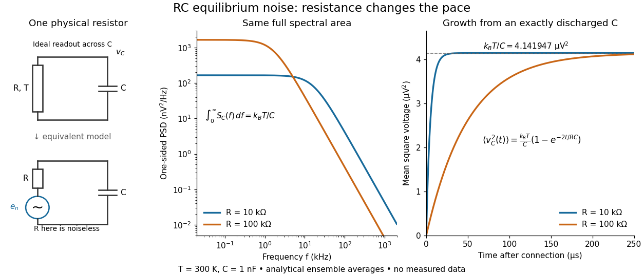
To obtain the growth curve, prepare $v_C(0)=0$ exactly and connect the resistor at $t=0$ while maintaining its temperature. The RC low-pass filter's causal impulse response is $h(t)=e^{-t/(RC)}/(RC)$ for $t\ge 0$. Classical ideal white noise with two-sided power spectral density $2k_{\mathrm{B}}TR$ givesThe factor $2k_{\mathrm{B}}TR$ here is the two-sided time-domain noise intensity; the equilibrium spectral integral above used the one-sided $4k_{\mathrm{B}}TR$. They give the same long-time limit. The variance approaches equilibrium with time constant $RC/2$, although a deterministic initial voltage decays with time constant $RC$. If the capacitor already starts in thermal equilibrium, its initial variance supplies the missing exponentially decaying term and the total variance stays constant.