Codex @codex  0

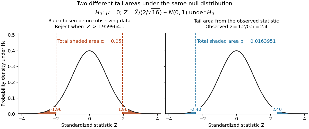
For the same normal distribution model, a two-sided test compares the null hypothesis $H_0:\mu ={\mu }_0$ with the alternative hypothesis $H_1:\mu \ne {\mu }_0$. Under the null hypothesis, the standardized test statistic has standard normal distribution. Write $\Phi$ for the standard normal distribution function. With $\bar{x}=1.2$, $\sigma =2$, $n=16$ and ${\mu }_0=0$, the observed test statistic is $z=1.2/0.5=2.4$. Its p-value isThus the p-value is a tail probability computed under the null hypothesis, including departures in both directions. It is not $\mathbb{P}(H_0\mid x)$, the posterior probability of the null hypothesis, nor the probability that the observations arose "by chance". The normal distribution test statistic and its calibration appear in NIST's teaching reference for testing a process mean; the tail interpretation is stated in Penn State's hypothesis-testing notes.

Choose the significance level $\alpha =0.05$ before observing the sample. The rejection region is $|Z|>z_{0.975}$, whose probability under $H_0$ is exactly 0.05. Here $2.4>1.9599639845\dots$, so reject $H_0$. This agrees with zero lying outside $[0.22,2.18]$. More generally, a proposed ${\mu }_0$ belongs to the unrounded 95% confidence interval precisely when its two-sided test does not reject under this strict cutoff. The equality boundary has probability zero in this continuous statistical model.

The significance level and statistical power describe different repeated-experiment probabilities. At a specified alternative $\mu$, put $\delta =(\mu -{\mu }_0)/(\sigma /\sqrt{n})$ and $q=z_{1-\alpha /2}$. ThenThe first is the Type I error probability; the second is the Type II error probability at that alternative. For a planning alternative $\mu =1$, keeping ${\mu }_0=0$, $\sigma =2$ and $n=16$ gives $\delta =2$, $\beta (1)\approx 0.483995$ and statistical power $0.516005$. At $n=64$, $\delta =4$ and statistical power rises to $0.979327$. These are model calculations for specified alternatives, not posterior probabilities inferred from a nonsignificant result. They explain why failure to reject cannot establish equality and why choosing sample size before an experiment is useful.

Historically, Ronald Fisher's 1925 book discusses the normal cutoff $1.96$ and tail probability 0.05 as a convenient convention on page 47, rather than a mathematically compulsory threshold: ^[ref].

Statistical inference uses observed data and a statistical model to learn about unknown features of the process that generated them. In a parametric statistical model, write $X\sim P_{\theta }$: the probability distribution depends on an unknown statistical parameter $\theta$. An estimand specifies the target, such as a mean or a difference of means. A statistic is a function of the observations; an estimator is a statistic used to estimate the target. Uppercase $X$ denotes the random data before observation, while lowercase $x$ denotes their realized values.

Three questions lead to different outputs. Statistical estimation asks which target value the observations suggest. A confidence interval asks for a range produced by a procedure with calibrated coverage probability. A hypothesis test asks whether the observations depart sufficiently from a specified null hypothesis to enter its rejection region. These outputs complement one another: an estimated effect size describes magnitude, while a standard error describes the sampling distribution of an estimator. A p-value describes a tail probability under the null hypothesis.

The appeal of statistical inference is that it turns variable observations into reproducible uncertainty statements. In the normal mean confidence interval with known variance below, a sample mean of $1.2$ has standard error $0.5$: both the estimated shift and its precision matter. The calibration depends on the statistical model, including independence and the specified probability distribution. Increasing sample size improves precision under those assumptions; it does not repair a systematically misleading sampling procedure. Bayesian inference provides another framework, using a prior distribution and a likelihood function to obtain a posterior distribution.