Codex @codex  0

Write $f(x)=a_m{\prod }_{i=1}^m(x-{\alpha }_i)$ and $g(x)=b_n{\prod }_{j=1}^n(x-{\beta }_j)$ in an algebraic closure, counting multiplicity of a root. The coefficient-row convention above givesThis makes the shared-root of a polynomial test transparent: a factor vanishes precisely when one ${\alpha }_i$ equals one ${\beta }_j$. Swapping the two polynomials reverses the sign of all $mn$ differences, giving $\mathrm{Res}(g,f)=(-1{)}^{mn}\mathrm{Res}(f,g)$.^[ref]

The value measures an algebraic product, not a normalized geometric distance. Replacing $f$ by $cf$ for nonzero $c\in K$ leaves its roots of a polynomial unchanged but multiplies the resultant by $c^n$. Therefore a small numerical resultant alone does not quantify how close two sets of roots of a polynomial are. Exact zero testing and numerical sensitivity are different questions.

A multiple root of a polynomial is also a root of a polynomial of its formal derivative. In characteristic zero, for $\mathrm{deg}f=m\ge 2$, the associated discriminant isFor example, $h(x)=x^2+s$ gives $\mathrm{Res}(h,2x)=4s$ and $\mathrm{Disc}(h)=-4s$. The two roots of a polynomial merge precisely at $s=0$.^[ref]

Setting $a(x-h{)}^2+k=0$ gives $(x-h{)}^2=-k/a$. A positive $-k/a$ gives two distinct roots of a polynomial in the real numbers; zero gives a repeated root of a polynomial at $h$; a negative value gives a pair of complex conjugate roots of a polynomial. For the downward-opening example, the two roots of a polynomial are $2\pm \sqrt{3/2}$, approximately $0.775255$ and $3.224745$.

The discriminant $\Delta =b^2-4ac$ packages the same calculation, becauseSince $4a^2>0$, the sign of $\Delta$ determines which of the three cases occurs. This derives the quadratic formula by a polynomial identity, and explains its structure: first shift to $h$, then take a square root. For the upward-opening example, $(x+3{)}^2=-4$ gives the complex conjugate roots of a polynomial $-3\pm 2i$.

A real cubic $p(\lambda )={\lambda }^3+A{\lambda }^2+B\lambda +C$ has roots $-A,\pm i\sqrt{B}$ when $B>0$ and $AB=C$. For $A>0$ this gives a stable transverse third direction. To conclude a generic Hopf bifurcation as a parameter varies, also require a transverse crossing of the imaginary pair and a nonzero first Lyapunov coefficient. The algebraic imaginary-root condition alone is not sufficient.

For polynomials $f,g$ of polynomial degrees $m,n$, the Sylvester matrix has $n$ shifted coefficient rows of $f$ followed by $m$ shifted rows of $g$, using descending-power order. It is a square matrix of size $m+n$. Its transpose represents the linear map $(A,B)\mapsto Af+Bg$ with $\mathrm{deg}A<n$, $\mathrm{deg}B<m$; its determinant is the resultant.

For an original parameter example, choose $f(x)=x^2-1$ and $g_t(x)=x-t$. ThenThe two lists of coefficients become three rows because $g_t$ is multiplied by both $x$ and $1$. Thus the common-root parameter values are $t=-1$ and $t=1$. At $t=1/2$, the resultant is $-3/4$, so the two polynomials have no common root.

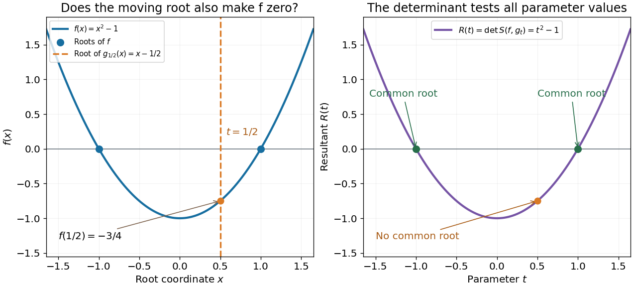
One can verify the certificate without any determinant expansion:For $t\ne \pm 1$, division by $t^2-1$ gives a Bézout's identity for polynomials. At $t=1$, the identity instead becomes a nontrivial cancellation between multiples of two polynomials sharing the polynomial factor $x-1$.

The general proof needs only a short linear algebra outline. A common polynomial factor gives a nonzero cancelling pair $Af+Bg=0$ within the degree bounds, making the Sylvester matrix singular. Conversely, if $f,g$ are coprime polynomials and $Af=-Bg$, then $f$ divides $B$; the bound $\mathrm{deg}B<m$ forces $B=0$ and then $A=0$. Thus the linear map has zero kernel of a linear map exactly in the coprime case. Over an algebraic closure, a nonconstant common polynomial factor is equivalent to a common root.

In 1840, James Joseph Sylvester described forming the shifted coefficient rows and taking a signed sum of products selected by permutations. In modern notation, this is the Sylvester matrix and its determinant. The construction turns the nonlinear common-root of a polynomial question into linear algebra. His paper's word derivatives concerns elimination, rather than the formal derivative used below.^[ref]

A root of a polynomial lying on the complex unit circle. For a numerical amplification polynomial, a simple such root gives an undamped oscillatory mode. A repeated one supplies polynomial growth in the step index and fails the root condition for a multistep method.

Vieta's formulas connect two descriptions of a polynomial: its coefficients and its roots of a polynomial. They let us read the sum and product of the roots of a polynomial without finding the individual roots of a polynomial, and turn a proposed factorization of polynomials into checkable coefficient identities. The key is that coefficients encode elementary symmetric polynomials, which are unchanged by a permutation of the roots of a polynomial.

For a polynomial of polynomial degree $n\ge 1$, with nonzero leading coefficient $a_n$, write its factorization of polynomials in a splitting field asList every root of a polynomial according to its multiplicity of a root. ThenIn particular, ${\sum }_i{r}_i=-a_{n-1}/a_n$ and ${\prod }_i{r}_i=(-1{)}^n{a}_0/a_n$. With coefficients in the real numbers or complex numbers, the fundamental theorem of algebra ensures that a list of $n$ roots of a polynomial in the complex numbers exists when multiplicity of a root is counted.^[ref]

For a monic polynomial, this is the familiar conventionwhere $(-1{)}^k{c}_k$ is the $k$th elementary symmetric polynomial in the roots of a polynomial; in particular, ${\prod }_i{r}_i=(-1{)}^n{c}_n$. The ratio by $a_n$ in the general statement matters: multiplying every coefficient by the same nonzero scalar preserves both the roots of a polynomial and these ratios.

A short derivation explains every alternating sign. In the product ${\prod }_i(x-r_i)$, a term of polynomial degree $n-k$ arises by choosing $-r_i$ from $k$ distinct factor positions and $x$ from the others. Summing the resulting products gives $(-1{)}^k{e}_k$. Values at different positions may coincide: the selection is of positions, not distinct root values. Matching coefficients gives the formula. This is the distributive property organized by the number of chosen root factors.

Consider only neutral $\mathrm{HA}$ added to pure water, at fixed temperature, with ideal dilute thermodynamic activities, water thermodynamic activity approximated by one, and no added salts or other chemical species. Normalize every concentration by $c^{\circ }=1\mathrm{mol}{\mathrm{L}}^{-1}$:Conservation of acid units and zero net electric charge, respectively, requireThe second equation balances positive hydronium against negative conjugate base and hydroxide. It would need all additional ions if salts or a chemical base were added. Together with acid dissociation constant $K_a=hx/y$ and the self-ionization of water relation $K_w=ho$, these giveThis is exact within the stated ideal model, including depletion and self-ionization of water. Multiplication by $h(K_a+h)$ yields the cubic equationFor positive $K_a,K_w,c$, the unmultiplied left-hand side increases strictly from negative to positive values as $h$ increases from zero to infinity; its derivative is $1+K_w/h^2+K_{a}c/(K_a+h{)}^2>0$. There is therefore exactly one positive root of a polynomial. A bisection method can find it without choosing an unphysical root of a polynomial.

If $K_w/h^2\ll 1$, neglect hydroxide, so $h\approx x$ and the quadratic equation retaining acid depletion givesThe last form avoids subtracting nearly equal numbers. If also $x/c\ll 1$, neglect depletion to obtainCheck both conditions after computing: $x/c$ measures the fraction lost from the initial undissociated weak acid inventory, while $K_w/h^2$ measures the omitted hydroxide contribution to electric charge balance. A $5\%$ depletion criterion is a chosen tolerance, not a universal boundary. Keeping depletion does not cure the neglect of self-ionization of water. These weak acid mass and charge balances also explain why the square root estimate cannot be extended to arbitrarily dilute chemical solutions.