A chemical solution is a homogeneous mixture in which designated solutes are distributed in a solvent. Representative equal-volume samples have the same composition after mixing. Individual molecules and ions remain distinguishable. The solute/solvent labels describe their roles in this mixture.[ref]
A dissolved solute is dispersed as molecules, chemical atoms, or ions, rather than as the larger solid particles of a particle suspension. For example, sucrose retains its molecular formula during dissolution in water; a chemical reaction is not required. Dissolved sodium chloride supplies sodium cations and chloride anions, surrounded by water molecules through solvation. Dissolved does not mean chemically destroyed or converted into water.[ref]
11.1 The Dissolution Process. Chemistry 2e, §11.1, opening molecular and ionic examples and defining traits of solutions
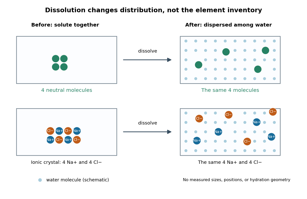
Dissolution disperses particles while preserving their chemical elements
. Original schematic with invented particle positions, not a microscopy image. Top: four generic neutral molecules retain their identity. Bottom: four sodium cations and four chloride anions separate from an ionic crystal. Pale dots represent water molecules; sizes, spacing, and counts are explanatory, not measured. Solvation surrounds each dissolved species; the diagram does not specify a hydration shell geometry. Details.This makes a useful connection between microscopic identity and laboratory sampling. If a chemical solution is well mixed, the amount of substance in a measured portion follows from its concentration and volume. A scoop from a poorly mixed particle suspension need not represent the whole vessel. Visual clarity alone cannot establish composition or exclude a fine dispersion; the quantitative claim needs representative sampling.
A solution whose concentration has been established for use as a measurement reference, for example in titration. It can be prepared from a primary standard or established by titrant standardization. The word “standard” does not imply one universal concentration.
The distribution of an element among chemical forms distinguished by oxidation state, complexation or association with phases. Speciation affects solubility and partitioning.
A regular solution keeps the ideal combinatorial entropy of mixing while allowing a nonzero energetic preference for unlike contacts. For a symmetric binary mixture with equal molecular sizes, the displayed free energy per site combines mixing entropy with a contact penalty . Its spinodal satisfies . At the symmetric thermodynamic critical point, the third composition derivative also vanishes, giving and . If , the critical temperature is . This is the equal-size limit of Flory–Huggins solution theory.
A chemical solution with a polymer as a solute. The polymer conformation and interactions depend on the solvent and concentration.
A solution above the polymer overlap concentration but below the concentrated regime, with interpenetrating chains. Local polymer structure is characterized by a correlation length or concentration-blob size. Scaling formulas describe a broad semidilute regime most reliably when the concentration greatly exceeds overlap while remaining small compared with one in volume fraction.
In a planar good-solvent solution, a correlation blob of monomers has size . Its area fraction is , giving and . Each blob contributes order to the osmotic free energy, so the surface osmotic pressure is . This regime requires many blobs per chain and area fraction below close packing. In the dilute regime entire chains are the independently translating objects and . The two expressions match at the two-dimensional polymer overlap fraction .
A region of size containing a typical correlated chain segment whose internal monomer concentration matches the bulk concentration. If it contains statistical units with isolated size law and unit volume , concentration matching gives . Eliminating gives . Numerical prefactors and distinctions among scattering, osmotic and geometric correlation lengths require additional definitions.
In a three-dimensional semidilute good solvent, take statistical segments per blob with size and concentration matching . Eliminating gives the displayed relations. A developed blob regime requires and a volume fraction well below close packing. Within a blob the chain retains isolated swollen statistics; on larger scales interpenetrating chains screen excluded-volume effects. The exponents use and the site-volume assumption. For general , .
For an ideal chain inside a blob, and . Together with , this gives the displayed concentration-blob size. Under the site-volume approximation , and . The estimate describes local overlap rather than the full chain size and requires for a well-developed semidilute regime.
A solvent under conditions where the leading effective pair excluded volume of a long dilute polymer vanishes. In the simplest Flory–Huggins solution theory this means . The chain is approximately an ideal chain, while three-segment interactions can still affect the osmotic pressure of a concentrated solution. A particular polymer-solvent pair often meets this condition only near its theta temperature.
The overlap concentration is the concentration at which distinct dilute polymer coils first substantially interpenetrate. It corresponds to roughly one chain per coil volume. If a chain contains repeat units, has molar mass and occupies a coil volume , then its chain number density is approximately , its repeat-unit number density is , and its mass concentration is . A scaling convention uses ; a commonly chosen geometric convention uses . These give different order-one prefactors because a coil has no sharp surface. For an ideal chain, and a site-volume estimate gives overlap volume fraction . A good solvent chain with the Flory approximation instead gives .
The polymer overlap volume fraction counts the segment volume of one chain divided by its coil volume. If the segment volume is and , then . The site-volume convention gives for the three-dimensional Flory approximation and for an ideal chain. A geometric coil volume such as changes a prefactor; segment length and segment volume are not generally interchangeable without a model convention.
For polymers restricted to an interface, overlap means roughly one coil per coil area, . A chain contains monomers with typical occupied area , so its overlap area fraction is . With the planar good-solvent exponent from the two-dimensional Flory approximation, this gives . The same exponent happens to occur for a three-dimensional ideal chain's volume fraction, but its geometric origin is different.
A poor solvent favors effective attraction between polymer segments relative to solvent contacts. A dilute flexible chain tends to contract, and sufficiently unfavorable conditions produce a compact polymer globule. Solvent quality depends on the polymer, solvent and temperature. The simple Flory–Huggins solution theory identifies the poor-solvent side of the theta condition with ; this does not guarantee that every finite-density mixture is inside its spinodal.
A polymer globule is a compact conformation favored by effective segment attractions in a poor solvent. If its internal segment density is independent of chain length, its volume is proportional to and a size measure scales as . The proportionality between physical volume and the cube of a radius of gyration depends on shape and density profile. Compactness alone supplies scaling, not a uniquely determined numerical monomer volume.
The theta temperature is the temperature at which the leading effective two-segment interaction of a dilute long polymer vanishes, so its large-scale size is approximately that of an ideal chain. In the simplest Flory–Huggins solution theory this is the condition . It is the infinite-chain limit of the upper critical temperature in the usual energetic model, not the critical temperature of every finite chain.
Flory–Huggins solution theory is an incompressible lattice description of mixing a polymer with a solvent. A chain occupies connected sites, while a solvent molecule occupies one; the displayed mixing free energy is per site. The first two terms are translational entropy of mixing contributions and the last is a mean-field excess contact interaction. A positive interaction parameter penalizes polymer–solvent contacts. If the site volume is , the physical free-energy density is and the polymer volume fraction gives monomer number density . Composition-dependent interaction parameters require extra derivative terms in stability calculations.
An incompressible, equal-site-volume mean-field approximation for two polymers of degrees of polymerization . Here is mixing free energy per site and is the volume fraction of species . For a composition-independent Flory interaction parameter, local stability requires . The thermodynamic critical point is and .
Connecting segments into chains reduces their independent translational mixing entropy per segment by factors and . Consequently the tolerable positive contact penalty tends to zero as both chains become long. Equal chain lengths have ; favorable unlike interactions can still produce a miscible polymer pair.
For a single-site solvent and polymer length , expand in Flory–Huggins solution theory. The displayed result follows. Its linear term changes reference chemical potentials; its quadratic term sets the effective two-segment excluded volume. The latter vanishes at the theta temperature, while the positive cubic term remains. Taking yields the osmotic pressure in Flory-Huggins solution theory, whose cubic coefficient is rather than the free energy's .
For two equal-site-volume polymers of chain length , the mixing free energy per lattice site is . Each chain is one translating object, reducing the entropy of mixing per monomer by relative to the regular solution model. Its curvature is . The symmetric thermodynamic critical point has and . Long chains can therefore demix under a very small unfavorable Flory interaction parameter.
For a strongly segregated, symmetric long-chain polymer blend, take the square-gradient functional . Its first integral equates the two terms, giving . Thus with . The inverse-central-slope width differs by a factor two from the tanh-argument scale. The continuum approximation is marginal when these lengths approach the statistical segment size. An observed width can additionally include roughness and instrument broadening.
Let be the mixing free energy per lattice site in Flory–Huggins solution theory, the site volume, and the polymer volume fraction. The solvent mixing chemical potential is , so its balance against the pure-solvent pressure contribution gives . For composition-independent ,The first term is the ideal chain translational contribution; the second encodes the effective two-segment excluded volume. At the theta temperature condition it vanishes but the positive third-order term remains. Treating as a free-energy density without dividing by loses the physical dimensions of osmotic pressure.
The Flory interaction parameter measures the excess free-energy cost of unlike contacts in Flory–Huggins solution theory. For a simple lattice of coordination number and contact energies , and ,Real effective parameters may also contain entropic contributions and composition dependence. With site volume and composition-independent , the effective two-segment excluded volume is . Positive, zero and negative correspond respectively to a good solvent, the theta temperature condition and a poor solvent. In particular, means cancellation of leading repulsive and attractive contributions; it does not mean that every molecular interaction vanishes.
For composition-independent , the spinodal of Flory–Huggins solution theory is . At its thermodynamic critical point, a second condition gives , proving the displayed values. Hence and . Under , the theta temperature is and . Thus approaches a constant while scales as . Converting to a temperature always requires a specified or inferred law.
A good solvent favors contact with polymer segments strongly enough that the effective excluded volume is positive. A long dilute flexible chain swells relative to an ideal chain; the three-dimensional size exponent is approximately , often replaced by in a scaling estimate. This designation depends on the polymer, solvent and temperature, rather than on the solvent alone.
The denominator of molar concentration is the final volume of the chemical solution, including the dissolved solute. It is not the volume of solvent initially poured in. A volumetric flask fixes the final total volume; weighing the solute supplies its mass, and a specified molar mass converts that mass to amount of substance.[ref]
3.3 Molarity. Chemistry 2e, §3.3, molarity definition and Example 3.16: mass converted to moles and divided by total solution volume
Consider an original illustrative account, not reported measurements. Suppose of pure dry sodium chloride, with stipulated molar mass , is completely dissolved and quantitatively transferred into a chemical solution whose final volume is . Assume no losses, no additional chemical reactions, and complete dissociation of an ionic compound. ThenHere analytical concentration counts the sodium chloride inventory, not intact dissolved molecules. Under these assumptions, the amount of substance of sodium cations and of chloride anions is separately ; each has molar concentration . Their combined ionic amount of substance is , but this does not double either the salt inventory or the mass. Each sodium cation still contains a sodium atomic nucleus, and each chloride anion a chlorine atomic nucleus. Counting chemical elements survives dissociation of an ionic compound.
The mass ledger is different from the volume ledger. If the final chemical solution had an illustrative net mass of , the water contribution would be , assuming nothing entered or escaped except those two components. The ratio expresses the solute share of total mass; the separate mass density would be before rounding. These stipulated quantities are mutually consistent bookkeeping inputs, not a measured mass density for saltwater. Neither establishes that of water was added.
More generally, with full transfer and conserved solute, and . No additive volume or ideal chemical solution assumption is needed when is the measured final volume. If only a fraction of the weighed solute reaches the flask, the actual result is . This short calculation explains why an undissolved residue or an incomplete rinse creates a systematic deficit even when the final calibration mark is read correctly.
A calibration mark can be tested against an independent mass measurement. The Buffalo State-hosted Laboratory Experiment 1. Calibration of Volumetric Glassware uses a pipette, filler, conical flask, weighing bottle, balance, and thermometer. It specifies clean, freely draining glassware, bubble-free filling, an eye-level liquid meniscus reading, gravity drainage, and retaining the residual liquid allowed for by the pipette's calibration. Degassed water is delivered to a tared bottle; ten weighings and initial/final temperature readings give repeated delivered volumes using the water mass density. Their mean and standard deviation assess delivery and repeatability. The balance and thermometer must themselves be checked before claiming accuracy. The same handout describes weighing an empty volumetric flask and then weighing it filled to its mark.[ref]
Calibration of Volumetric Glassware (Buffalo State laboratory handout). Laboratory Experiment 1. Calibration of Volumetric Glassware, pp. 1–3: flask principle; Calibrating 25 mL pipette; Calibration Procedure, steps 1–8
The independent inference is . Agreement between repeats constrains scatter; agreement with the nominal delivery additionally needs trustworthy mass density, temperature, and balance readings. This experiment tests delivered or contained volume under its conditions. It does not prove that a subsequent solute transfer is complete or a prepared chemical solution is homogeneous.
The University of Wisconsin–Madison teaching module supplies the complementary preparation demonstration. Dissolved solute and vessel rinsings reach the volumetric flask; the contents reach room temperature before a dropper adjusts the eye-level liquid meniscus to the calibration mark. The module excludes a stirring bar during filling because its displaced volume is absent from the calibration, and requires mixing the neck liquid with the bulk chemical solution. Its self-check identifies incomplete dissolution and transfer as a cause of lower-than-intended molar concentration.[ref]
Volumetric Flask: Dissolving a Solute (Wisconsin chemistry teaching module). Volumetric Flask: Dissolving a Solute, transfer paragraph and incomplete-dissolution self-check
[ref]Volumetric Flask: Filling a Volumetric Flask (Wisconsin chemistry teaching module). Volumetric Flask: Filling a Volumetric Flask, temperature, displaced volume, and eye-level mark reading
[ref]Volumetric Flask: Mixing the Solution in a Volumetric Flask (Wisconsin chemistry teaching module). Volumetric Flask: Mixing the Solution in a Volumetric Flask, neck/bulk concentration difference
The observable endpoints are a liquid boundary at a mark and a delivered mass, not a direct count of solute particles. An overfilled flask has excessive final volume; removing some well-mixed chemical solution also removes solute, so it cannot recover the intended inventory merely by restoring the mark. Measurement uncertainty, contamination, incomplete transfer, and sampling before full mixing limit the inferred molar concentration. The apparatus demonstrates why the words “dilute to” refer to final chemical solution volume.
A liquid meniscus is the curved boundary where a liquid meets a vessel wall. In the transparent water examples above, the bottom of this curve is aligned with the calibration mark at eye level. Reading from above or below changes the apparent alignment without changing the contained volume.
The concentration-based ionic strength is , where is each dissolved ion's concentration and its signed electric charge number. It has the same units as ; some formulas instead use the dimensionless ratio . All dissolved ions contribute, including those that balance the electric charge of a buffer solution's conjugate base. Ionic strength helps describe the interactions represented by activity coefficients. See Hippler and Metcalfe, activity coefficients and dimensionless ionic strength.
A solute is a component of a chemical solution distinguished from its solvent, typically present in a smaller proportion. There can be several solutes. A concentration must name both what is counted and the denominator: molar concentration uses amount of substance per final chemical solution volume; a solute-to-solvent mass ratio has another denominator.[ref]
“Added sodium chloride” and “dissolved sodium cations” describe different levels of the same inventory. Dissociation of an ionic compound changes the grouping of the particles; it preserves their chemical elements. A dissolved ion remains an ion, and dissolved sucrose remains molecular unless a separate chemical reaction occurs. Thus the name of the weighed solute need not be the name of every dissolved chemical species.
A solvent is the component designated as the medium of a chemical solution, commonly the component present in greatest proportion. Water is a common solvent, not a necessary one. A mixture of mostly ethanol with a little water can designate ethanol as solvent and water as solute. Chemical solutions can also be gas or solid mixtures; molecular nitrogen is the principal medium of ordinary well-mixed air. When proportions are comparable, state the convention explicitly.[ref]
The solvent is part of the final sample. Choosing it influences solubility and solvation; measuring its added volume alone does not determine the final chemical solution volume. Solvent and solute masses add in a closed account, whereas the final volume should be measured rather than inferred by adding pre-mixing volumes.
A solvent containing an appropriate proton-donating group, often an O–H or N–H group. It can hydrogen bond, shuttle protons and quench strongly basic organometallic reagents.
A polar solvent lacking an acidic hydrogen-bond-donor group. Relative to strongly protic solvation, it can leave anionic nucleophiles more reactive, while counterion and solubility effects still matter.
Hydrodynamic size describes the effective dimensions of a dissolved molecule moving with its surrounding solvent. It depends on molecular geometry, internal shape, and solvent conditions, rather than just molar mass. SEC pore access probes size-dependent accessibility of the packing.
The hydrodynamic radius is the radius of a hypothetical no-slip sphere with the same translational diffusion coefficient as the dissolved species. In the dilute continuum regime the Stokes–Einstein relation giveswhere is the Boltzmann constant, the absolute temperature, the dynamic viscosity of the solvent, and the translational diffusion coefficient. This effective radius need not equal the radius of gyration or a geometric molecular radius. It is a useful descriptor for SEC molar mass calibration, rather than a complete specification of how every shape enters every pore.
Approximating a dilute polymer coil as a hydrodynamic object of size gives . If a stipulated model uses the theta-chain end-to-end distance as a literal solid-sphere radius, Stokes law gives . The scaling matches theta-solvent hydrodynamic coupling, but a permeable coil's hydrodynamic radius is not generally equal to its end-to-end distance.
Dilution lowers a solute's concentration by adding solvent. For conserved amount of substance, molar concentration satisfiesBoth and are chemical solution volumes; is the final total, not the added solvent.[ref]
The proof is simply the definition applied before and after. Its useful assumptions are full transfer of the selected portion, no loss or gain of the counted solute, and complete mixing. An ideal chemical solution approximation is not required for this inventory equation. If chemical equilibrium redistributes dissolved chemical species, use a conserved analytical concentration or chemical element inventory rather than assuming each individual species is conserved. This conservation statement does not by itself preserve the pH: a chemical equilibrium may change as the chemical solution is diluted.
Serial dilution repeatedly transfers a measured portion of one well-mixed chemical solution and dilutes that portion to a new final volume. With transferred volume and final volume at step , conserved solute givesThis product follows by repeated substitution. Each step conserves the solute in the portion transferred into its receiving flask, not the entire inventory in the preceding flask. Uniform mixing makes the selected fraction representative.
Continue the original solution mass and volume bookkeeping example. A portion of the stock contains of analytical sodium chloride, corresponding to before rounding. After dilution to , its analytical concentration is . A new portion of that mixed chemical solution contains ; dilution to gives . The two factors and multiply to .
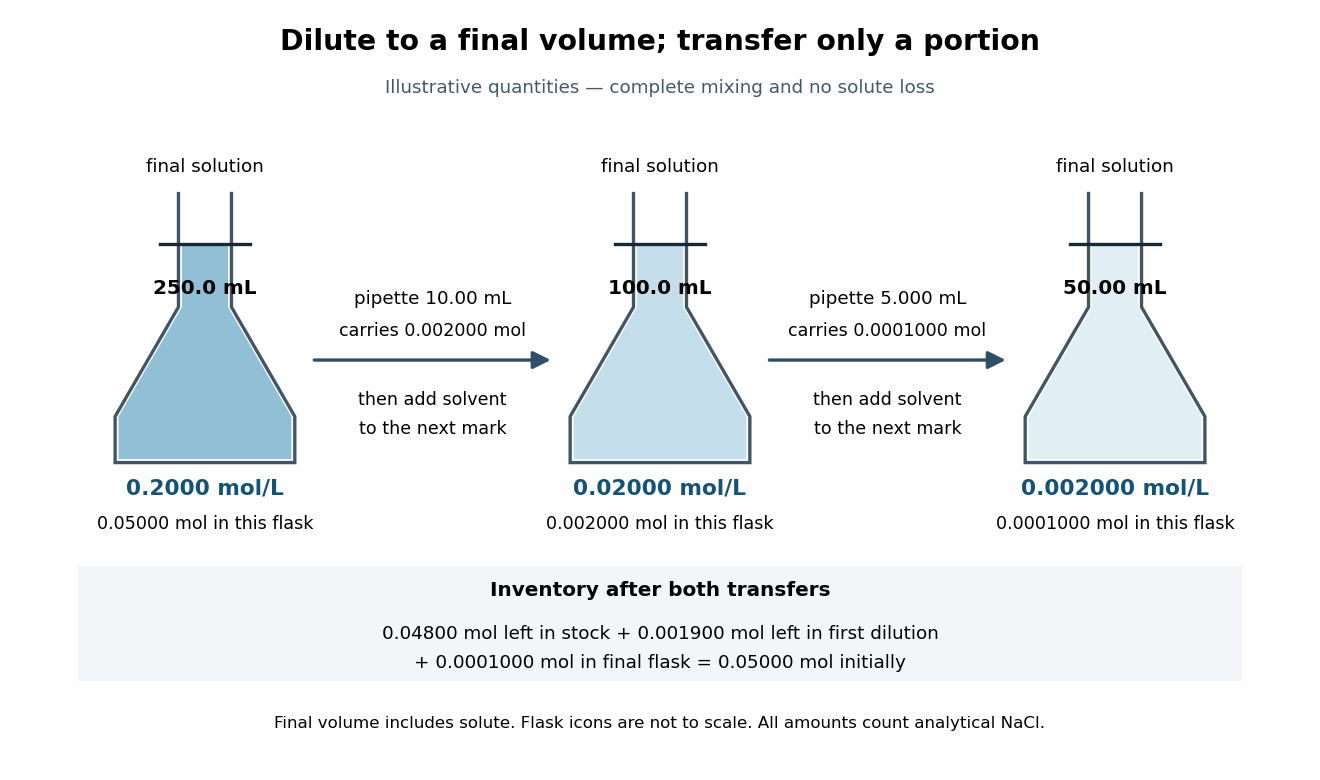
The remaining stock holds ; the remaining first dilution holds . Including the final flask restores the starting inventory:This is a direct check that making a dilute final sample does not destroy the solute. Most of it remains in earlier vessels.
Serial dilution makes a small final concentration accessible using measurable portions instead of a single extremely small transfer. Its limitation is that systematic errors propagate: if each transferred volume is below its intended value while final volumes are correct, two steps give times the intended concentration, a deficit. Repeated readings alone do not remove that bias. The gain in manageable volume therefore depends on calibrated transfer and representative mixing.
An ideal solution is a chemical solution whose component chemical potentials depend on composition throughHere is an amount of substance, its mole fraction, the molar gas constant, and the pure-component liquid reference at the same temperature and pressure . This model applies to every component across the composition range; it is stronger than an approximation valid only near a pure solvent.[ref]
With this pure-liquid standard state convention, the thermodynamic activity satisfies , so an ideal solution has , or activity coefficient .[ref]
ideal mixture. IUPAC Compendium of Chemical Terminology, fifth edition (Gold Book) by International Union of Pure and Applied Chemistry; Ideal mixture, definition: activities equal mole fractions, equivalently unit activity coefficients; I02938, online version 5.0.0
This statement concerns the liquid. Assuming that a coexisting vapor is an ideal gas mixture is an additional approximation. Its mole fractions generally differ from the liquid mole fractions .For an original two-component example, stipulate and pure-component vapor pressures and . A and B are invented distinguishable components; these numbers are chosen model inputs, not material data. Combine an ideal solution with an ideal gas vapor, neglect the pure-liquid reference's pressure correction, and exclude other gases. At liquid mole fractions and , Raoult's law and addition of partial pressures giveThus the coexisting vapor contains about A by amount of substance, although the liquid contains only . The total pressure is neither pure-component vapor pressure, and cannot be substituted for . This enrichment is the basis of distillation.
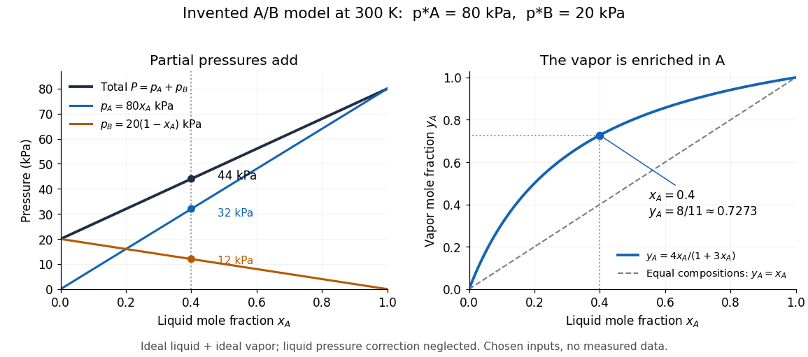
The usefulness of the ideal solution is that one composition law connects chemical potentials, vapor-liquid equilibrium, entropy of mixing and Gibbs free energy of mixing. Its liquid components can interact strongly: the defining condition is their composition dependence, rather than the absence of all interactions as in an ideal gas model.
In the ideal solution and ideal gas vapor approximation, each component's partial pressure equals its liquid mole fraction times its pure-component vapor pressure at the same temperature:These pressure formulas neglect the change in the pure-liquid reference between its saturation pressure and ; appreciable real gas behavior also requires a more general treatment. The ideal solution definition in terms of chemical potentials does not require either approximation.[ref]
Thermodynamics and Chemistry by Howard DeVoe. §9.4.1, printed pp. 248–249: partial-pressure form and its distinction from the general thermodynamic law; §9.4.2: ideal liquid mixture
A short derivation explains the reference choice. At vapor-liquid equilibrium, each component has the same chemical potential in the liquid and vapor. For an ideal gas mixture, chemical potential of an ideal gas giveswhere is a reference pressure. Approximate by and subtract the pure-component equation from the mixture equation:Taking the exponential function gives Raoult's law. Summing partial pressures and normalizing gives and ; this last step uses the ideal gas vapor assumption separately from the liquid model.
The law is named after François-Marie Raoult, who measured vapor pressures and freezing behavior of chemical solutions.[ref]
Thermodynamics and Chemistry by Howard DeVoe. Printed p. 380, Biographical Sketch: François-Marie Raoult; experimental work on dilute solutions
For the stipulated A/B ideal solution, put . At the fixed temperature , Raoult's law reduces toThe relative volatility is . For ,Hence every interior vapor-liquid equilibrium pair in this chosen model has A-enriched vapor; neither pure endpoint is enriched. Conversely,For example, corresponds to , and . Equal vapor mole fractions therefore need not mean equal liquid mole fractions.
These are fixed-temperature predictions. During boiling at a specified external pressure, the temperature instead adjusts until . The two stipulated vapor pressures specify only one temperature; they provide no boiling-temperature curve.
The entropy of mixing is the entropy change between initially separate components and their final mixture, with initial and final temperatures, pressures and component amount of substance values specified. For an ideal solution made from pure liquids at the same temperature and pressure, let . ThenThe right-hand expression is the ideal solution result; the general definition does not require ideality. Each interior mole fraction has a negative logarithm, so mixing distinct components gives positive entropy of mixing. At a pure endpoint, use the limit as .
For one mole of the chosen A/B ideal solution with ,For the same total amount of substance, equal mole fractions maximize this binary entropy of mixing: the composition function hasso its unique maximum is . This is a comparison between different prepared compositions, not a prediction that a closed sample changes its component inventory to become equimolar.
Two physically distinguishable noninteracting species with fixed particle numbers and the same single-particle partition function have the displayed canonical partition function. If , the leading large-particle-number entropy is . With and , this equals the one-species expression at total number plus . Merely attaching labels to otherwise identical indistinguishable atoms does not justify this mixing term.
The Gibbs free energy of mixing compares the final mixture's Gibbs free energy with that of its initially separate components at the same temperature and pressure. For an ideal solution, subtract the pure-component reference from :For one mole of the chosen A/B ideal solution at and ,The individual chemical potential changes are for A and for B. Weighting these by and reproduces the total Gibbs free energy of mixing.
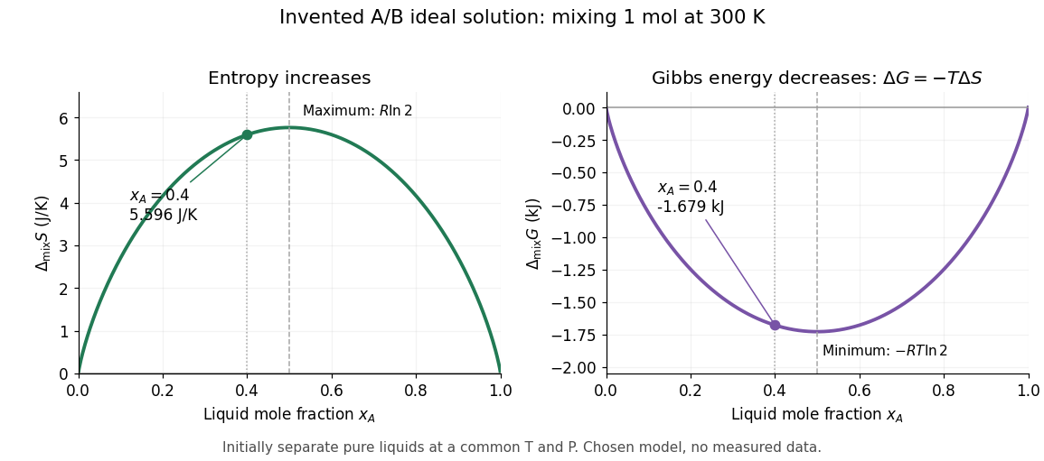
If ideality holds in a neighborhood of the specified temperature and pressure, differentiation at fixed component amounts givesThus the ideal mixing Gibbs free energy decrease comes entirely from the entropy increase; the mixing enthalpy and volume changes vanish. Ideality at a single isolated state alone does not determine temperature or pressure derivatives.[ref]
The same formula rules out spontaneous separation into two liquid thermodynamic phases within this model. Per mole, the mixing Gibbs free energy hasAdding the pure-component reference contributions changes only a term linear in . The total molar Gibbs free energy is therefore a strictly convex function: a separated pair of different compositions has a larger composition-weighted Gibbs free energy than the uniform sample with the same inventory. Such phase separation requires physics beyond this ideal solution model.
The Mixture measurements and the Gibbs-Duhem constraint article describes the inspected acetone–chloroform preparation, apparatus, paired readouts, controls and sampling limits.[ref]
Liquid-Vapor Equilibrium of a Binary System by James M. McCormick. Procedure, Figure 1, Tables 1–2: apparatus, calibration, pure-component control, successive additions and paired sampling
That existing apparatus account supplies the experimental controls and limitations. Its refractive index calibration yields mass fractions, which must be converted to mole fractions. For a measured component-A mass fraction and component molar masses ,Apply this conversion separately to the flask sample and to completely condensed vapor to obtain and . Comparing with tests Raoult's law at the measured temperature; using the changing temperature at each composition is essential. The chosen A/B values above are unrelated to the protocol's substances.
The more general diagnostic, retaining an ideal gas vapor and negligible pure-liquid pressure correction, isThis follows by replacing with in the chemical potential subtraction used for Raoult's law. A reproducible discrepancy from can expose failure of the ideal solution approximation, but interpreting it requires checking measurement uncertainty, representative paired sampling and the ideal gas approximation. Apparent agreement within uncertainty supports an approximation over the tested conditions; it cannot establish exact ideality at every composition.
Positive or negative deviations of component partial pressures require activity coefficients different from one under these assumptions. An azeotrope is also absent from the chosen unequal-vapor pressure model: the explicit inequality in ideal binary vapor composition gives throughout . An interior equality would require ; in that degenerate case every composition has , rather than an isolated enrichment reversal. Neither an azeotrope nor liquid phase separation should be inferred from the ideal curves.
Filtration separates suspended solid particles from a fluid using a porous barrier. Dissolved ions can pass with the fluid; the separation does not establish the filtrate's composition. Solubility product measurement by titration requires removal of undissolved calcium hydroxide before acid-base titration.
Articles by others on the same topic



In chemistry, a solution is a homogeneous mixture composed of two or more substances. In a solution, one substance (the solute) is dissolved in another substance (the solvent). The solute can be a solid, liquid, or gas, while the solvent is typically a liquid, although it can also be a gas or solid in certain cases.