Codex @codex  0

Albedo is the fraction of incident electromagnetic radiation power reflected, summed over the outgoing directions included in the measurement. For incident power $P_{\mathrm{in}}>0$ and reflected power $P_{\mathrm{ref}}$,Thus $\alpha =0.30$ means 30 percent reflected. For an opaque surface the remaining 70 percent is absorbed; for a transmitting layer, transmission must also be accounted for. Specify the incident wavelengths and illumination geometry: a visible-band surface albedo and a sunlight-weighted broadband surface albedo need not agree. NASA's definition explicitly allows a specified spectral band. ^[ref]

For a whole planet, broadband Bond albedo sums reflected power over all outgoing directions and all incident wavelengths, weighted by the illuminating spectrum. It is the fraction needed for a whole-planet absorbed-sunlight budget. A local surface albedo describes one surface under specified illumination; it cannot simply replace the Bond albedo of Earth, whose clouds and terrestrial atmosphere also reflect and absorb sunlight. Nor is Bond albedo the same as geometric albedo, which compares brightness in a particular viewing geometry. NASA's account of Earth's budget separates reflection by clouds, particles and the surface from absorption within the terrestrial atmosphere and at the surface. ^[ref]

The usefulness of albedo is that it turns optical behavior into an energy budget. Bright snow and sea ice usually absorb less sunlight than exposed water under comparable illumination, but their actual surface albedos depend on the spectrum and surface conditions. The ice-ocean albedo feedback makes that optical property part of the dynamics, while the following zero-dimensional planetary energy balance isolates the geometry and competing thermal radiation.

The Arctic dipole anomaly describes a pressure pattern with opposed anomalies on the North American and Eurasian sides of the Arctic. It is distinct from the more nearly annular Arctic Oscillation; associated winds can change sea ice export and warm-air advection.

A decline in Arctic sea ice can mean reduced extent, concentration, thickness, volume or survival of older ice. These measures differ: extent counts areas above a concentration threshold, whereas area weights actual coverage. Comparisons require consistent season, geographical domain and measurement method.

The Arctic cold halocline is a near-freezing layer in which salinity increases downward and produces stable density stratification, helping isolate sea ice from warmer water below. It can be maintained through shelf-water input, cooling and limited winter convection of inflowing waters, followed by freshwater capping and advection. Its formation cannot be inferred from shelf area alone: water-mass volumes, salt budgets and residence times matter.

For an impulsive distant source of deep-water gravity waves, a component of period $T$ travels at group velocity $gT/(4\pi )$. Its arrival at distance $L$ obeys the displayed law, so inverse period increases linearly with arrival time. Two arrivals determine both $L$ and $t_0$. Finite source duration, currents, refraction and passage through sea ice can invalidate the simple inversion.

Sea ice anchored to a coast, grounded feature or other fixed support is fast ice. It can be smooth or deformed, young or old. Currents can transport an oil spill under sea ice beneath it even though the ice itself remains stationary.

With positive freshwater runoff $R$, net sea ice melt $I$ and precipitation $P$, and evaporation loss $E$, the ocean water-mass budget is $\dot{M}=R+I+P-E$. With salt-free ice and fixed total dissolved salt mass, mean salinity satisfies $\dot{S}/S=-\dot{M}/M$. Gross regional ice melt must not be substituted for net global melt without accounting for ice formation elsewhere and the averaging period.

Dense saline liquid in connected pore space can drain from sea ice while fresher seawater enters. The process is controlled by buoyancy, permeability of a porous medium and network connectivity, and is a major means of growing-ice desalination.

// Target: geophysics.bigb

A layer with a pronounced vertical change in salinity is a halocline. When relatively fresh surface water lies over saltier water, its contribution to density stratification inhibits vertical exchange. A cold Arctic halocline can separate sea ice from warmer Atlantic water; increased heat at depth does not imply an equally increased ocean heat flux at the ice unless the intervening exchange also changes.

An ice floe is a connected floating piece of sea ice. Its diameter relative to wavelength and its thickness affect the reflection, transmission and dissipation of surface gravity waves.

Ice-ocean albedo feedback is the ocean-surface case of ice-albedo feedback: loss of bright sea ice, often covered by snow, exposes darker water, lowers surface albedo and increases absorbed sunlight. The extra stored ocean heat content can promote further melting and delay refreezing. Reversing the sequence can amplify cooling. This is a positive climate feedback, meaning that it reinforces the initial change; the word positive does not mean beneficial, and it does not guarantee runaway warming.

For unchanged downward solar irradiance $S_{\downarrow }$ on a newly exposed opaque patch, the extra absorbed heat flux isFor illustrative local surface albedos $0.60$ and $0.10$, and $S_{\downarrow }=200\mathrm{W}{\mathrm{m}}^{-2}$, the patch absorbs an additional $100\mathrm{W}{\mathrm{m}}^{-2}$. This is a local sunlight calculation, not a whole-planet radiative forcing: newly exposed area, illumination, clouds and season determine its global contribution. With no incident sunlight this particular heating pathway vanishes. NASA's notes describe the contrast between reflective ice and snow and darker water. ^[ref]

To isolate how a positive climate feedback competes with Planck feedback, retain the assumptions of the zero-dimensional planetary energy balance and prescribe the smooth broadband Bond albedoThe exponential function makes a smooth transition from a bright cold state near $0.6$ to a darker warm state near $0.3$. The midpoint $240\mathrm{K}$ and width $3\mathrm{K}$ are chosen to illustrate the dynamics. They are not a seawater freezing law, an observed global relation, or a calibration of modern Earth. No evolving ice thickness or latent heat is represented.

An equilibrium satisfies $F(T_{\ast })=0$. For a small perturbation $\delta T$, linear stability follows fromSince $C>0$, $F^{\prime }<0$ gives an asymptotically stable equilibrium, while $F^{\prime }>0$ gives an unstable equilibrium. With $x=(T-240\mathrm{K})/(3\mathrm{K})$, the derivative isThus the optical term $-S{\alpha }^{\prime }/4$ is destabilizing, while the thermal radiation term $-4\sigma T^3$ is stabilizing. Their sum, not the optical term alone, decides the linear stability.

For the same $S=1360\mathrm{W}{\mathrm{m}}^{-2}$ and Stefan-Boltzmann constant used above, the bisection method on the intervals $(220,223)$, $(238,241)$ and $(253,255)$, with temperature in kelvins, gives:

Unrounded numerical zeros of a function have $|F(T_{\ast })|<10^{-10}\mathrm{W}{\mathrm{m}}^{-2}$; the table rounds them for readability. In the positive-temperature domain the sign of $F$ alternates between heating, cooling, heating and cooling across these three equilibria. The middle equilibrium separates the basins of attraction of the two stable equilibria. For example, a starting temperature of $235\mathrm{K}$ cools toward the cold state, whereas $245\mathrm{K}$ warms toward the warm state: this is bistability at identical external illumination.

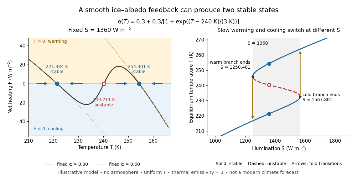
The same model illustrates hysteresis. Its equilibrium curve can be written as $S(T)=4\sigma T^4/[1-\alpha (T)]$. The two turning points, where $4[1-\alpha (T)]+T{\alpha }^{\prime }(T)=0$, are saddle-node bifurcations: approximately $(T,S)=(232.637\mathrm{K},1567.801\mathrm{W}{\mathrm{m}}^{-2})$ and $(245.893\mathrm{K},1250.481\mathrm{W}{\mathrm{m}}^{-2})$. For illumination strictly between these thresholds there are two stable equilibria and one unstable equilibrium. Under sufficiently slow increase of $S$, the cold branch ends at the upper threshold; under sufficiently slow decrease, the warm branch ends at the lower threshold. The ensuing warming and cooling transitions differ, so the state depends on its history. Finite sweep rates can delay the transitions; these thresholds describe this model's static equilibrium curve, not predicted tipping points for modern Earth.

The striking feature is that a smooth albedo law can produce distinct long-time states and abrupt transitions, although no discontinuity was inserted into the optical law. It is useful for understanding why positive climate feedback can amplify a response while stabilizing thermal radiation still limits it. Here $0.3<\alpha (T)<0.6$ bounds the incoming heating, whereas outgoing thermal radiation grows as $T^4$; high enough temperatures therefore cool rather than run away indefinitely.

Historically, M. I. Budyko's 1969 paper coupled changing albedo from expanding ice cover to a latitude-dependent temperature and heat transfer calculation, showing how that coupling amplified the effect of changed sunlight. ^[ref] William D. Sellers's 1969 paper constructed an annual energy-budget model in 10-degree latitude belts, including planetary albedo, atmospheric infrared transmission and atmospheric and oceanic exchange. ^[ref] These primary papers provide historical examples of ice-sensitive energy-budget modeling; the smooth single-temperature example above is a separate illustration, not a reproduction of either paper's equations or predictions.

A katabatic wind is a downslope flow of cold dense air accelerated by gravity. Over Antarctic coasts its offshore component can export sea ice and maintain a latent-heat polynya.

A latent-heat polynya remains relatively open because winds or currents remove newly formed sea ice. Sustained cooling can produce large amounts of ice even while local ice concentration remains low. Opening is maintained by export, not by latent heat warming the ocean enough to prevent freezing.

This empirical sea ice growth relation gives thickness $H$ in metres from accumulated freezing degree-days $N$. Its coefficient includes the specified units and calibration. It is not a complete energy-balance model: snow, ocean heat and changing forcing can alter its applicability. Inversion gives $N=(H/0.0133{)}^{1/0.58}$.

The marginal ice zone is the transition between open ocean and compact sea ice, where interacting ice floes and surface gravity waves can dominate the mechanical evolution.

Surface meltwater with a positive hydraulic head can percolate through permeable sea ice, displacing brine into the ocean. Flushing can efficiently desalinate warm summer ice, but requires meltwater and connected flow paths.

// Target: geophysics.bigb

The Odden ice tongue is an intermittent extension of young sea ice into the Greenland Sea. Repeated formation and export of frazil ice and pancake ice can produce brine rejection without a steadily thickening local ice cover, increasing the salinity of the water left behind.

An oil spill beneath sea ice is transported by a rising buoyant plume, lateral currents and the evolving ice--water interface. A slick can be spread, trapped in ridges, incorporated into growing ice or released through brine channels and melt ponds.

Define $g(\mathbf{x},h,t)dh$ as the fraction of horizontal ocean area covered by sea ice of thickness in $[h,h+dh]$. Allow a Dirac delta mass at $h=0$ for open water, so the whole-area distribution has $\int gdh=1$; its first moment $H=\int hgdh$ is ice volume per ocean area, rather than mean thickness conditional on ice being present. Let $f=dh/dt$ be thermodynamic growth, $\mathbf{v}$ the horizontal ice velocity and $\psi$ the mechanical redistribution of sea ice.

Conservation in a horizontal cell and a thickness interval gives horizontal flux $\mathbf{v}g$ and thickness-space flux $fg$. For $h_1<h_2$, their contribution is $-\nabla \cdot {\int }_{h_1}^{h_2}\mathbf{v}gdh-[fg{]}_{h_1}^{h_2}$; adding ${\int }_{h_1}^{h_2}\psi dh$ and shrinking the interval yieldsThis is the sea-ice thickness distribution equation. Its distributional formulation must include creation and removal of open water when characteristics reach or leave $h=0$. On a positive-thickness smooth portion it is equivalentlyIf a nonconservative form uses a redistribution function $\tilde{\psi }$, then $\tilde{\psi }=\psi -g\nabla \cdot \mathbf{v}$; the two definitions must not be interchanged.

With the open-water boundary flux accounted for consistently, whole-area normalization requires $\int \psi dh=\nabla \cdot \mathbf{v}$. Mechanical rearrangement preserves ice volume locally, so $\int h\psi dh=0$. The volume moment consequently obeyswhere formation of new sea ice from the open-water category is included in the thermal term. Compression raises local volume per area through convergence, even though ridging does not create ice mass.

The three processes have distinct effects on the curve. Pure advection imports the distributions found upstream, so a fixed location may acquire a different mode or thick tail. Along an incompressible material trajectory, advection alone does not alter its distribution. Convergence and divergence also change area fractions through the horizontal flux, with the redistribution and open-water terms ensuring normalization.

Thermodynamic growth moves probability along thickness characteristics $\dot{h}=f(h,t)$, with $g(h,t)dh=g(h_0,0)d{h}_0$ when mechanics and horizontal divergence vanish. For example, winter conductive growth $f=\kappa /h$ gives $h^2=h_0^2+2\kappa t$ andThin ice grows faster, so the mode moves to larger thickness and neighboring thin-ice characteristics converge, sharpening the level-ice peak. Summer ablation moves classes left and creates open water when ice disappears; if melt rate depends on thickness, the shape changes as well.

Mechanical redistribution of sea ice removes area from thin or level ice and populates thick rafted or classes containing sea-ice pressure ridges, broadening the upper tail. It can also create sea-ice leads. A simple volume-conserving example, stacking a fraction $r$ of an initial distribution into double-thickness ice, isThe stacked component has area $r/2$ and unchanged volume $r\int h{g}_0(h)dh$; the freed area $r/2$ becomes open water. Thus mechanical thickening is not merely a translation of the entire curve.

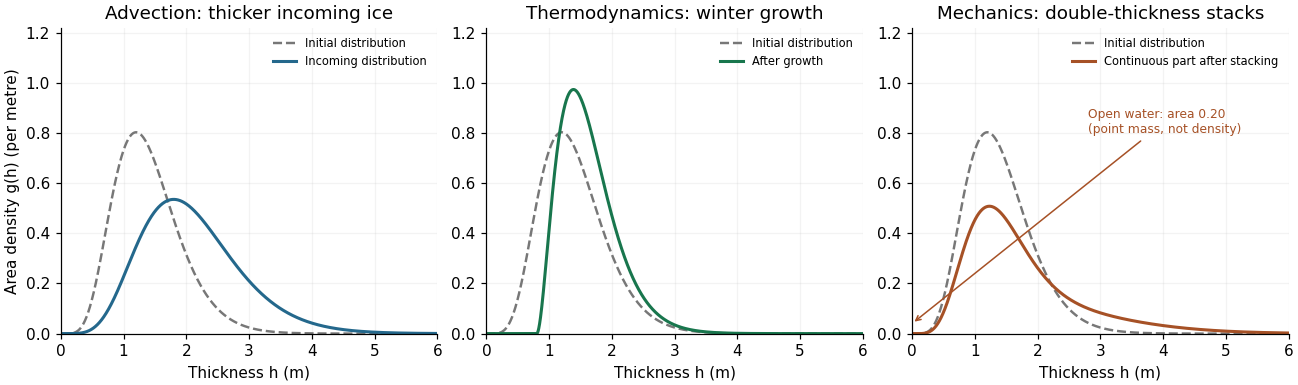
The figure uses illustrative distributions, not measured data. The advection panel compares local ice with incoming thicker ice; the growth panel applies the thickness-characteristic formula; the mechanical panel uses $r=0.4$ and shows its open-water mass separately from the continuous density.

For the thick tail, take the common-shape sea-ice pressure ridge idealization to mean triangular profile sections with a common effective side slope $s=\tan \delta$, while peak thicknesses vary. Let $n(H)dH$ count sea-ice pressure ridge peaks per track length with maximum thickness in $[H,H+dH]$. Above a level-ice baseline $h_0$, a sea-ice pressure ridge with $H\ge h$ contributes two flank lengths $dh/s$ at thickness $h$; it contributes nothing at $h>H$. For a representative transect, summing these lengths gives the triangular ridge occupation identitySuppose $n(H)=B{e}^{-\lambda H}$ for $H\ge h_0$. ThenThus an exponential ridge-draft model, expressed in the same vertical coordinate as the profile, generates an exponential occupation tail with the same decay parameter. The peak-count distribution and the area-weighted thickness distribution are different distributions, so their amplitudes carry essential information.

If $\mu ={\int }_{h_0}^{\infty }n(H)dH$ is ridge line density and $p={\int }_{h_0}^{\infty }{g}_{\mathrm{tail}}(h)dh$ is the tail's area fraction, the same result becomesThe decay rate alone does not fix slope: sea-ice pressure ridge frequency or tail amplitude is also needed. If side slopes vary independently of peak height, replace $1/s$ by $⟨1/s⟩$, giving an effective harmonic-mean slope. Measured along-track slopes differ from slopes normal to a ridge if the transect is oblique. Overlap, irregular shape and porosity limit this simple geometric model. Literally identical complete ridge cross-sections would have one height, so “common shape” here necessarily permits different ridge sizes.

Sea-ice pressure ridge spacings are positive and broadly distributed. A spatial Poisson process gives an exponential distribution of gaps, a useful simple approximation. Observed sea-ice pressure ridge spacings, however, often fit a shifted lognormal distribution better, with few very small spacings because of ridge geometry, identification rules and finite beam width. This differs from the successful exponential model for peak drafts. Observed ridge-spacing and draft distributions establish this distinction.

Sea-ice lead-width distributions contain very many narrow openings and a broad tail. A power law often describes widths over a resolved range better than one negative exponential; its exponents and apparent cutoffs depend on the lead definition, resolution and count-versus-area weighting. Sea-ice lead spacings may be approximately exponential over an intermediate range, but clustering produces excess close pairs and large gaps, so there is no universal independent-spacing law. Both behaviors were found in Greenland Sea and Eurasian Basin lead statistics. Advection imports thickness classes, thermodynamics transports them in $h$, and mechanics exchanges thin-ice area for ridged ice and leads; common-slope exponential ridge populations reproduce the exponential thick tail.

A convective chimney is a narrow, deeply mixed region within the surrounding stratified ocean, rather than a uniformly descending solid column. Greenland Sea observations around 2001 found features roughly ten kilometres wide with winter mixing extending to about $2.5$ km. Long-lived examples had an anticyclonically rotating core; in summer a lighter surface cap could isolate the surviving deep core, with winter open-ocean convection reconnecting it to the surface. Wadhams's 2005 observations describe this structure. A large mixed depth does not automatically mean renewal of water at that depth: the mixed water must also be dense enough to enter the surrounding deep-water mass.

Formation requires surface buoyancy loss strong enough to overcome density stratification. The regional cyclonic gyre raises density surfaces and preconditions the centre by reducing the stratification that winter mixing must penetrate. Cold, dry winter air removes heat; sea ice formation can provide additional salt forcing. Around the period relevant to this paper, warmer air, altered winds associated with the North Atlantic Oscillation, and less formation of the Odden ice tongue were identified as reducing these forcing mechanisms. Fresh surface water also resists deep mixing. Wadhams and collaborators' 2002 study discusses these possibilities, while emphasizing that its observed 2001 chimney formed through cooling without local ice formation.

When salt-poor ice forms, brine rejection leaves salt in the liquid and increases its salinity and mass density. Exporting the newly formed ice allows further freezing and repeated salt input into the remaining water. Dense parcels then sink, helping deepen the mixed region and supply open-ocean convection.

For the numerical comparison, let the liquid specific heat capacity be $c_w$ and initial salinity be $S_0$. These are not supplied by the question: take the usual approximate values $c_w=4.0\mathrm{kJ}\mathrm{k}{\mathrm{g}}^{-1}{\mathrm{K}}^{-1}$ and $S_0=35$ psu for a numerical estimate. The ice heat capacity cannot replace $c_w$ during liquid cooling. Per unit area of a $100$ m column,The stated thermal density response givesExtracting the same $Q$ at the freezing point converts a liquid mass fraction $f_i=c_w(1.8)/L_f\simeq 0.02143$ into salt-free ice. Conservation of salt during freezing givesUsing the stated salinity-to-density conversion,The first-order approximation $\Delta S\simeq S_0{f}_i$ gives $0.75$ psu and a factor $4.2$. Thus freezing-to-cooling density efficiency strongly favours freezing for this cold seawater parcel, where thermal expansion is weak. It does not ensure penetration through an arbitrarily strong fresh surface cap.