Codex @codex  0

Erosion or displacement of the cold halocline weakens the barrier separating sea ice from warmer water below. It can therefore increase the upward ocean heat flux without requiring a large new warming of that deeper water. Wind-driven mixing, changes in shelf-water supply, and freshwater redistribution can alter the halocline. This mechanism couples the Atlantic heat reservoir to atmospheric and circulation changes.

Warmer Atlantic water increases the reservoir of heat beneath the Arctic surface layer. However, stable density stratification across the cold halocline often prevents that heat from directly reaching the ice. The effect on sea ice depends on upward mixing and ocean heat flux, with greater direct access in some Atlantic-influenced regions; a temperature increase at depth alone is insufficient to quantify basal melting.

The mechanisms affect surface energy input, heat supply from below, and the transport and thickness of sea ice. They reinforce one another: atmospheric warming and ocean heat thin the cover; circulation can export old ice; thinner ice melts earlier, increasing open-water absorption and strengthening ice-albedo feedback. Heat below the cold halocline matters only to the extent that mixing delivers it upward. Consequently the seven effects cannot be assigned independent percentages from the information given; their importance varies by region and year.

In a forward-looking answer from the paper's 2009 context, sustained warming would be expected to produce continued Arctic sea ice decline, a longer summer open-water season, less multi-year sea ice, and potentially nearly ice-free late summers within coming decades. Winter darkness permits new first-year sea ice to form, so loss of summer ice does not imply immediate year-round disappearance. Winter ice would tend to become thinner, more seasonal, and slower to recover after enhanced ocean heating. A precise date requires a forcing scenario and model, and internal variability causes year-to-year departures. Wang and Overland's 2009 projection is a contemporary example of such a conditional summer outlook.

Open water absorbs more sunlight than bright sea ice, and melt ponds also lower the surface albedo. More absorbed heat promotes further melt and can be stored in the upper ocean, delaying autumn freezing. This ice-albedo feedback amplifies an initially forced loss during the sunlit season. Perovich and collaborators' 2008 measurements identify solar heating of the upper ocean as the main heat source for enhanced bottom melting in their observed Beaufort Sea case. Feedback is especially important locally after open water develops; it does not supply solar heat during polar winter.

Long-term thinning lowers the latent heat inventory that must be supplied before a patch of sea ice disappears. Thin ice is also more mobile and vulnerable to mechanical breakup. A smaller fraction of multi-year sea ice therefore increases susceptibility to a warm or windy summer. Thin ice grows relatively rapidly in winter because it conducts heat more readily, giving a stabilizing response that partly opposes continued thinning without cancelling sustained warming.

The Arctic Oscillation changes pressure patterns and winds, redistributing sea ice and altering export through Fram Strait. Removing thick old ice and replacing it with thinner new ice preconditions greater summer loss; winds also open leads and change ocean circulation. This is an important dynamic contributor and source of variability, rather than a universal one-to-one relation between the oscillation index and total summer ice extent.

The solar constant measures the incident power per area normal to the sunlight. A spherical Earth of radius $R$ intercepts sunlight over the disc $\pi R^2$, but radiates over its surface $4\pi R^2$. For uniform surface albedo $a$ in the global energy-budget approximation, absorbed power is $(1-a)S\pi R^2$. Treat the surface as a blackbody, assume efficient heat redistribution and neglect internal heating. The Stefan–Boltzmann law and the planetary surface energy balance then giveFor a nonuniform surface the same power balance instead defines an effective planetary equilibrium temperature, $T_E^4=⟨T^4⟩$; its fourth root is not generally the arithmetic mean of the local temperatures. Also, area-averaging the surface albedo is an approximation to the properly insolation-weighted averaging. These are the simplifications implicit in the naked-planet calculation.

Take $R=6.371\times 10^6\mathrm{m}$, so $A_E=4\pi R^2=5.10\times 10^{14}{\mathrm{m}}^2$. The changed area is $A_i=10^{12}{\mathrm{m}}^2$, givingThe initial planetary equilibrium temperature is $T_0=254.8\mathrm{K}$. ThusThe differential estimate $\Delta T\simeq -T_0\Delta a/[4(1-a_0)]$ gives the same result. This is the global equilibrium response of the specified model, not the immediate local Arctic warming or the full atmospheric response.

The exceptional 2007 Arctic sea ice decline is best understood as a weather event acting on an already vulnerable ice cover, with several reinforcing pathways. Warmer air increases downward long-wave heating, lengthens the melt season and delays autumn freezing. Changes in snowfall and the development of melt ponds also change the surface energy balance. Air temperature alone, however, does not identify the source of the observed bottom melt: heat must reach the underside through the ocean.

Warmer Atlantic-origin water supplies a larger subsurface ocean heat content after entering through Fram Strait and the Barents Sea. Its influence on sea ice depends on vertical exchange, because a cold, relatively fresh halocline normally separates it from the ice. Erosion of that halocline, through altered freshwater distributions, wind-driven mixing or changes in circulation, weakens stable density stratification and can increase upward ocean heat flux. A warmer Atlantic layer without this exchange need not produce immediate extra bottom melt. Conversely, warmer Pacific inflow through Bering Strait introduces heat into the shallower western Arctic; advection through the Chukchi Sea provides another route to ice retreat and ocean heat storage.

The Arctic Oscillation changes winds, ice motion and export. Positive phases during earlier years helped remove old, thick ice through Fram Strait and left a younger, thinner pack. Summer 2007 also had a pronounced pressure contrast between the Beaufort region and the Eurasian Arctic, associated with the Arctic dipole anomaly. Its winds promoted ice displacement and warm-air transport. The summer circulation should not be described merely as a particular Arctic Oscillation index: the spatial pattern and the preconditioning from earlier years both matter.

Long-term thinning reduces the latent heat of fusion needed to remove the remaining ice. Replacement of multi-year sea ice by first-year sea ice therefore makes a given summer heat input more effective, while mobile thin ice is more readily redistributed or exported. These dynamical changes can expose open water early enough for substantial solar absorption. Water and melt ponds have lower surface albedo than snow-covered ice, so absorbed short-wave energy rises, increasing upper-ocean heat storage and bottom melt. This ice-ocean albedo feedback also delays refreezing. In the Beaufort Sea in 2007, enhanced solar heating of the newly exposed upper ocean was an especially important explanation of extreme bottom melt. Thus thinning and wind-driven opening can initiate retreat, while solar heating amplifies it; changes in Atlantic or Pacific heat supply can further reinforce the process where circulation permits.

A further positive climate feedback involves terrestrial carbon. Loss of the insulating ice cover permits greater autumn and winter transfer of stored ocean heat to the atmosphere. The resulting regional warming can increase thaw of coastal and inland permafrost. Microbial decomposition of previously frozen organic material then releases carbon dioxide, and oxygen-poor wet environments also release methane. These greenhouse gases strengthen the greenhouse effect, increasing global warming and further thaw. The permafrost carbon feedback provides the causal chain from summer ice retreat to an additional global influence. An Arctic methane feedback involving subsea sources is also possible, but the amount actually reaching the atmosphere depends on oxidation and transport; an abrupt, wholesale release is not a necessary consequence of summer ice loss.

For the bottom-melt estimate, use ${\rho }_i=917\mathrm{kg}{\mathrm{m}}^{-3}$ and the given $L_f=336000\mathrm{J}\mathrm{k}{\mathrm{g}}^{-1}$. Assume the ice at the melting interface is already at its local freezing temperature; there is then no separate sensible-heating term. Per square metre the latent heat requirement isJuly through September has $92$ days, so the mean ocean heat flux to the ice isUsing ${\rho }_i\simeq 900\mathrm{kg}{\mathrm{m}}^{-3}$ instead gives about $76\mathrm{W}{\mathrm{m}}^{-2}$, within the intended accuracy. Around the date of this examination, the estimated net anthropogenic radiative forcing since preindustrial times was about $1.6\mathrm{W}{\mathrm{m}}^{-2}$; doubling carbon dioxide gives about $3.7\mathrm{W}{\mathrm{m}}^{-2}$. The calculated bottom flux is tens of times larger. There is no energy-budget contradiction: it is a local, summer ocean-to-ice heat transfer, supplied by absorbed sunshine, stored heat and transport, whereas radiative forcing is a global perturbation to the radiation budget. Redistribution and local absorption can produce much larger regional fluxes than the global forcing.

For an already ice-free $100\mathrm{m}$ water column, take ${\rho }_w=1025\mathrm{kg}{\mathrm{m}}^{-3}$ and liquid-water specific heat capacity $c_w\simeq 4000\mathrm{J}\mathrm{k}{\mathrm{g}}^{-1}{\mathrm{K}}^{-1}$. Assuming all the same energy remains in that uniformly mixed column,If the water initially lies near the seawater freezing point, about $-1.8{}^{\circ }\mathrm{C}$, its final temperature is approximately $\boxed{-0.3{}^{\circ }\mathrm{C}}$. An absolute final temperature requires that additional initial condition; the energy calculation itself determines only the temperature increase. The given ice specific heat capacity is not the appropriate value for heating liquid seawater.

A steric sea level change is caused by a change of water volume at fixed ocean mass. Warming usually lowers seawater mass density, producing thermosteric sea level change; freshening also lowers density and produces a halosteric contribution. Both depend on the temperature, pressure and salinity dependence of the equation of state. Regional freshening or warming can therefore change local sea level even when the global ocean mass has not increased.

An eustatic sea level change concerns the ocean water amount or basin capacity. On the coming-century timescale, the principal positive mass contributions are melting mountain glaciers and ice caps, and loss of grounded ice from Greenland and Antarctica, including iceberg discharge. Terrestrial water storage also matters: groundwater depletion transfers water to the ocean, whereas reservoir filling retains it on land. Snowfall accumulation can partly compensate ice loss. Basin changes associated with geology matter over longer periods, and vertical land motion changes locally measured relative sea level. Melting floating sea ice has already largely displaced its eventual meltwater volume; its direct contribution is small compared with transfer of grounded ice into the ocean. Small density and salinity corrections do not alter that distinction.

For scale, a contemporary budget available in 2010 gave the following approximate contributions for 1993–2003, in $\mathrm{mm}\mathrm{y}{\mathrm{r}}^{-1}$:These are period-specific estimates with appreciable uncertainties, particularly for Antarctica, rather than exact closure of the budget. For comparison, over 1961–2003 the observed rate was about $1.8\mathrm{mm}\mathrm{y}{\mathrm{r}}^{-1}$ and the estimated thermal expansion contribution about $0.4\mathrm{mm}\mathrm{y}{\mathrm{r}}^{-1}$. The shorter interval need not define a permanent acceleration by itself, but the magnitudes show that thermal expansion and land-ice loss are both essential.

With continued warming, increasing ocean heat content sustains thermosteric sea level change, including after surface warming slows because the deep ocean equilibrates gradually. Increased ice ablation generally increases glacier runoff, although small glaciers eventually lose much of their available ice. Surface melt and changes in outlet-glacier flow can increase the ice-sheet contribution; ocean-driven loss of ice shelves can accelerate discharge of grounded ice. Greater snowfall provides some compensation but cannot be assumed to cancel these losses. Thus, under continued substantial greenhouse gas emissions, the global rate is likely to rise above its historical few millimetres per year, with an increasing contribution from the great ice sheets. The precise century-scale increase depends on emissions, ocean heat uptake and ice sheet dynamics; a single fixed rate extrapolated from one decade is inadequate.

For the idealized mixed-layer calculation, the stated density response givesAt fixed column mass, $\rho H=(\rho +\Delta \rho )(H+\Delta \eta )$, so to first orderThis is only the thermosteric sea level change from the prescribed layer and warming. The much larger total observed rise since the nineteenth century does not, by itself, prove deeper warming: part of that rise is eustatic sea level change. After independently allowing for the mass contribution, a larger remaining steric signal would require warming below $200\mathrm{m}$, a different temperature distribution, or corrections to the simplified equation of state. Direct temperature profiles do independently establish subsurface ocean warming. It reaches depth through winter mixing and open-ocean convection, especially in the North Atlantic and parts of the Southern Ocean; through subduction of surface waters into the interior; and through advection and turbulent mixing. Formation and spreading of intermediate and deep waters transmit surface properties far beyond the immediate region of heat uptake. Warm surface water need not simply sink locally: cooling, freshwater effects and density stratification govern the actual pathways.

Using $R=6.371\times 10^6\mathrm{m}$, the ocean area is $A_o=0.70(4\pi R^2)=3.57\times 10^{14}{\mathrm{m}}^2$. A liquid runoff volume $\Delta V=600\mathrm{k}{\mathrm{m}}^3=6.00\times 10^{11}{\mathrm{m}}^3$ givesThis is the contribution from that input, before allowing for other exchanges in the global ocean freshwater budget.

For the sea-ice dilution estimate, the ocean volume is $V_o=A_o(4000\mathrm{m})=1.428\times 10^{18}{\mathrm{m}}^3$. Let its initial mean salinity be $S_0$; the question does not specify it, so use $S_0\simeq 35$ psu for a numerical estimate. Interpret the $600\mathrm{k}{\mathrm{m}}^3$ as liquid freshwater-equivalent melt, with ${\rho }_f\simeq 1000\mathrm{kg}{\mathrm{m}}^{-3}$. Salt mass remains fixed while liquid water mass increases, givingConsequentlyApproximating the densities as equal gives $-1.47\times 10^{-5}$ psu per year. If the quoted volume instead denotes literal solid-ice volume, use ${\rho }_i\Delta V$ for the added mass; with ${\rho }_i=917\mathrm{kg}{\mathrm{m}}^{-3}$ the result is $-1.32\times 10^{-5}$ psu per year. Either convention gives the same order of magnitude. Floating-ice melt can change mean ocean salinity even though its direct sea-level effect is small: displaced volume and dissolved salt concentration are different budgets.

An observed net freshening is a statement about the sum of all freshwater exchanges, not a separate measurement of every positive contribution. Let $M$ be liquid ocean mass, $R$ net freshwater runoff from land, $I$ net global sea-ice melt minus formation, and $P-E$ net precipitation minus evaporation, all expressed as masses per unit time. The global ocean freshwater budget and salt conservation giveThe runoff term must include non-ice river input as well, or those other exchanges must already have been netted out. If the measured freshening equals that predicted from $I$ alone, positive runoff is still possible providedor an equivalent compensating term exists in the complete budget. For instance, excess evaporation can remove water at the same rate at which land-ice runoff supplies it; compensating net ice formation elsewhere must also be included if $I$ was initially only the Arctic contribution. Gross seasonal melt cannot be compared with an annual global trend without subtracting refreezing. Such compensation also means that the runoff-only sea-level increment need not equal the total retained increment. If runoff is additional, sea-ice melt is already net and global, and every other freshwater term is zero, the two contributions must add: under those stronger assumptions the alleged equality would be inconsistent. The apparent paradox is resolved by closing the complete freshwater and salt budgets.

A polynya is a persistent or recurrent area of open water or relatively thin ice within an otherwise ice-covered region. Persistence of the opening does not mean absence of ice formation: a latent-heat polynya can continuously make ice and export it. In contrast, a sensible-heat polynya remains open because ocean heat inhibits freezing. Both processes may occur at the same site.

At an Antarctic coast, cold air descending from the elevated continent produces strong katabatic winds. Their offshore component drives sea ice away from a fixed coastline, fast-ice edge or grounded-iceberg barrier. Open water exposed to the cold atmosphere loses heat rapidly; frazil ice forms, aggregates into pancake ice or consolidated new ice, and is exported offshore. The opening continues as long as export balances production. Headlands, the shelter provided by fast ice and the direction of the prevailing winds determine the location and size. Terra Nova Bay is a characteristic coastal example. Such latent-heat polynyas are ice factories rather than permanently warm holes in the ice pack.

At an ice shelf front the fixed boundary is floating shelf ice instead of land. Offshore winds blowing across the shelf can similarly remove newly formed sea ice, so an ice-front polynya need not have a different thermodynamic mechanism from a coastal one; the Ross Ice Shelf front provides an important wind-driven example. Shelf-front geometry, ice tongues, grounded icebergs and changes in calving alter the shelter and the supply of drifting pack ice. Some ice-front openings also receive significant sensible heat from currents, tidal mixing or upwelling, and heat carried out of an ice-shelf cavity can affect freezing. A sensible-heat polynya requires a sufficiently warm ocean supply, whereas the latent-heat mechanism requires continuing removal of the ice that does form. Consequently a strict identification of all coastal openings with one mechanism and all ice-shelf openings with the other would be incorrect.

The oceanic roles are substantial. Rapid heat loss and freezing produce brine rejection, raising shelf-water salinity and mass density. The resulting convection and circulation can carry dense shelf water into ice-shelf cavities; melting beneath an ice shelf modifies it into colder, fresher ice-shelf water. Dense shelf and cavity-modified waters can subsequently descend the continental slope, mix with adjacent waters and contribute to Antarctic bottom water. The outcome depends on bathymetry and the density after mixing: not all rejected brine reaches the abyss.

These localized regions can therefore have a disproportionate effect on deep-ocean ventilation, oxygen supply, carbon transport and the large-scale ocean circulation. They are also intense sites of ocean-to-atmosphere heat and moisture transfer. Seasonal sunlight arriving in open water supports high biological production where nutrients are available, with consequences for marine food webs and carbon cycling. Antarctic polynyas connect wind-driven ice export, concentrated ice production and dense-water formation; ice-shelf fronts add a floating boundary and possible cavity-related heat and freshwater exchanges.

Off northeast Greenland, the Northeast Water Polynya is organized by the interaction of local currents and winds with coastal geometry and relatively fixed ice barriers. A regional northward coastal current encounters the Norske Øer shelf-ice barrier; divergence and shelter on its lee side help create the southern opening. This local northward current should not be replaced in the explanation by assuming uniform southward flow along the entire Greenland coast. In summer, weak winds, the current and the barrier can maintain the opening, while solar heating and the seasonal heat budget allow it to expand northward without continuous new-ice formation.

Winter conditions differ. Strong northerly winds can remove newly formed sea ice from the northern region around Ob Bank, with the Ob Bank ice barrier and Kronprins Christian Land controlling shelter and divergence. Large air–sea temperature differences then sustain rapid freezing and export. Thus the recurring geographical opening has a changing balance of dynamical export and seasonal thermodynamics; long-lived does not mean identical formation conditions throughout the year. Ice barriers themselves can also change between years.

The North Water Polynya, or Pikialasorsuaq, occupies the Smith Sound and northern Baffin Bay region between Greenland and the Canadian Arctic. An ice arch across the narrow upstream channel restricts the arrival of thick drifting Arctic ice. Northerly winds and predominantly southward transport through the channel remove newly formed ice into Baffin Bay. The combination of blocked upstream ice supply and continuing downstream export maintains low ice concentration despite strong winter cooling. The location and stability of the arch therefore matter as well as the local wind. Warm Atlantic-origin water carried along the Greenland side can provide a sensible-heat contribution, with tidal and other mixing helping deliver heat upward; the entire opening should not be attributed either exclusively to warm-water convection or exclusively to wind.

Both regions permit much greater winter ocean-to-atmosphere heat transfer than nearby thick ice, and both can concentrate ice formation and brine rejection. The production of saline shelf water affects local density stratification and exchanges with surrounding waters; it is not automatically equivalent to deep or abyssal water formation. In spring and summer the early availability of light and open water promotes biological production and supports rich marine food webs. These persistent or recurrent openings also provide habitat and access of particular importance to Arctic animals and coastal communities. The key Arctic mechanisms are ice-barrier control of supply, current- and wind-driven divergence, and a seasonally varying contribution from ocean heat.

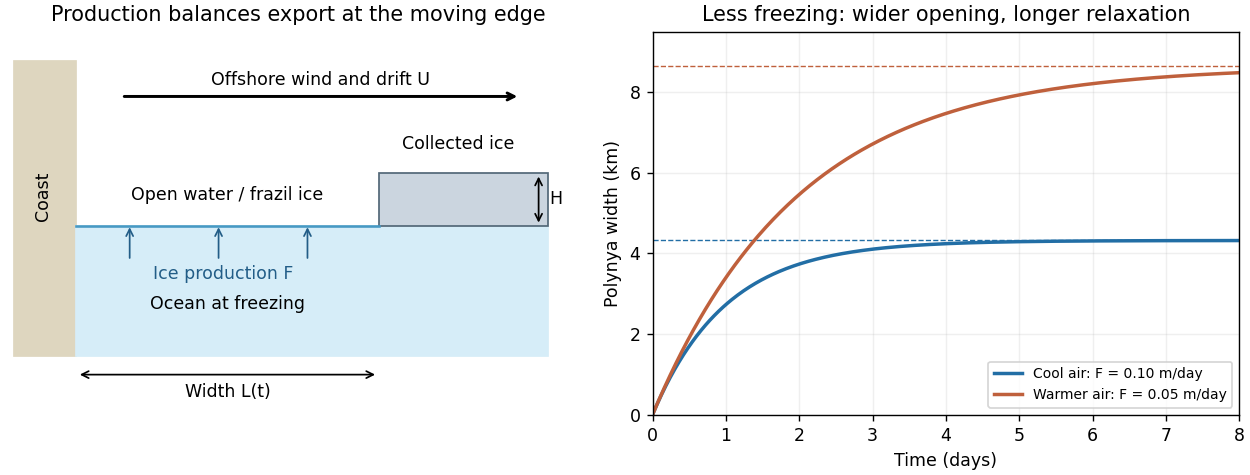
In the Pease polynya model, take a straight fixed coast at $x=0$ and an offshore polynya edge at $x=L(t)$. Let consolidated pack ice move offshore at speed $U>0$, let new ice be produced throughout the opening at equivalent thickness rate $F>0$, and let the collected ice at the edge have a prescribed thickness $H$. All fluxes below are per unit length of coastline. The new-ice volume production is $FL$, while the consolidated-ice export relative to the moving edge is $H(U-\dot{L})$. Neglect storage of drifting frazil ice inside the opening, so conservation givesThis is the simplest Pease closure: newly formed ice is collected at the edge rapidly enough that production can be equated to the instantaneous edge flux. A model retaining frazil storage would instead include the local balance ${\partial }_{t}h+{\partial }_x(uh)=F$, with frazil thickness $h$ and transport velocity $u$, together with an edge condition; it should not silently be identified with the instantaneous-collection approximation.

For constant $U,F,H$, the stable equilibrium and relaxation time areIn particular, an initially closed opening has $L(t)=L_{\infty }(1-e^{-t/\tau })$. It initially opens at speed $U$, then slows as its larger area produces more ice. It reaches $63\%$ of its ultimate width after $\tau$ and $95\%$ after $-\tau \log 0.05\simeq 3\tau$; the exact equilibrium is approached asymptotically, not reached at a finite opening time.

The production rate is determined by the energy budget. With $Q_{\mathrm{surf}}$ positive for net upward surface heat loss and $Q_o$ the heat supplied from the underlying ocean, water at its local freezing temperature givesThe surface loss includes sensible and latent turbulent transfers and net radiation. For example, the sensible component is approximately ${\rho }_a{c}_{p,a}{C}_{H}V(T_f-T_a)$, where $V$ is wind speed and $C_H$ an exchange coefficient. Ice motion is commonly parameterized as a small fraction of the offshore wind speed, but currents and the direction relative to the coast also matter. Thus colder air and stronger net cooling increase $F$ and narrow the opening; faster export increases $U$ and widens it; thicker collected ice increases both $L_{\infty }$ and $\tau$. Stronger winds can increase both export and heat loss, so the width's dependence on wind can be much weaker than the formula with artificially fixed $F$ would suggest.

The assumptions are steady spatially uniform forcing; a one-dimensional straight coast; fixed collection thickness and drift speed; no alongshore import of pack ice; water already at freezing rather than an appreciable sensible-heat reservoir; and negligible residence time of newly formed ice. Real coastlines, time-dependent winds, ocean currents, atmospheric adjustment over warm open water and variable ice accumulation can all violate these assumptions. The model describes a latent-heat polynya, not an opening maintained principally by a warm deep-ocean heat supply.

If air temperature rises while wind, $H$ and the other external parameters are unchanged, the smaller air–sea temperature difference reduces net heat loss and hence $F$. For $0<F^{\prime }<F$,The opening becomes wider and takes longer to attain the same fraction of its new equilibrium width. Its initial opening speed remains $U$; the longer equilibration follows from weaker ice production, rather than slower initial export. If warming eliminates net freezing, $F=0$ gives $L=L(0)+Ut$ in the simple kinematic closure, with no finite freezing-balanced width. A negative $F$ represents melt and is outside the positive-production Pease model.

For the shelf-water calculation, a $30$-day month at $0.05\mathrm{m}\mathrm{da}{\mathrm{y}}^{-1}$ produces $h_i=1.5\mathrm{m}$ of ice. Assume a well-mixed $D=100\mathrm{m}$ shelf column, no compensating advection or precipitation, and fixed ice and water densities ${\rho }_i=917$ and ${\rho }_w=1025\mathrm{kg}{\mathrm{m}}^{-3}$. The frozen fraction of its initial liquid mass isLet the liquid initially have salinity $S_0$, and newly formed ice retain $rS$ with $r=0.3$ and $S$ the instantaneous ambient value. For remaining liquid mass $M$, freezing removes salt with the departing ice, so conservation of salt with salt-retaining ice givesThereforeAn initial shelf-water salinity is needed for an absolute answer. Taking $S_0=34$ psu gives $\boxed{\Delta S\simeq 0.32\mathrm{psu}}$. At the accuracy of an equal-density thickness calculation, $f\simeq 1.5/100$ and $\Delta S\simeq 0.7S_{0}f$, giving about $\boxed{0.36\mathrm{psu}}$ for $S_0=34$ psu. These estimates describe the same modest increase. Treating ice as completely fresh would overestimate brine rejection by omitting the factor $0.7$.

The resulting water is denser and can leave the shelf and intrude beneath fresher surface water. It is therefore a physically plausible contribution to the cold halocline. Nevertheless, this one-month column budget yields only a few tenths of a psu, and the salinity contrast across the Arctic halocline can be several psu. If water from a shelf occupying one-third of the area were spread through an equally deep layer over the whole ocean, the average increase would be only about $0.1$ psu. This illustration is not a volume budget for the actual deep Arctic: shelf area fraction is not ocean water-volume fraction, and the exported water can be concentrated within a relatively thin halocline layer.

Consequently this calculation supports a shelf contribution but does not establish its dominance. Repeated seasonal ice production, enhanced production in polynyas, shelf-water export, freshwater dilution, and the thickness and residence time of the receiving layer would all be needed to test dominance. The assumption that the shelf initially becomes ice-free limits the first month's salt production; it does not bound an entire winter's cumulative production if new ice is continually removed.

Another pathway is winter cooling and limited convection of Atlantic-origin water as it enters the Arctic and encounters the ice-covered ocean. Cooling and local freezing can make it near-freezing water without requiring that it first be formed throughout the Siberian shelf. A subsequent fresh surface cap limits further convection; the cooled water is advected into the basin beneath that cap, producing a cold, salinity-stratified lower halocline. Pacific-origin waters also contribute to halocline structure in the western Arctic. Both formation and maintenance depend on circulation and freshwater supply, not simply on the presence of freezing somewhere. The strong stable density stratification then limits upward transfer of heat from the deeper Atlantic layer to sea ice.

The case for anthropogenic global warming rests on a physically consistent combination of forcing, energy storage and observed response, rather than on the claim that every unusual event has the same cause. For this examination, the observational comparison is the evidence available around 2010, and the two forecast horizons are approximately 2060 and 2110. Separating the robust mechanisms from uncertain regional details is essential to a coherent attribution of recent climate change.

The greenhouse effect follows from radiative transfer. Sunlight supplies energy, while the Earth loses energy mainly through long-wave radiation. Carbon dioxide, methane and other greenhouse gases absorb and emit in parts of that outgoing spectrum. Increasing their concentrations alters the levels and temperatures from which radiation escapes, initially reducing the net loss of energy for a given surface state. The surface and atmosphere must then warm until outgoing radiation again balances the input. Strong absorption near the centres of some bands does not eliminate the influence of additional gas: absorption in the wings and the changing height of emission still matter. For scale, the approximate carbon dioxide forcing law $\Delta F\simeq 5.35\log (C/C_0)\mathrm{W}{\mathrm{m}}^{-2}$ gives about $3.7\mathrm{W}{\mathrm{m}}^{-2}$ for doubling. It describes a forcing, not the ultimate temperature response, which additionally involves climate feedbacks and ocean heat uptake.

Measured increases in atmospheric carbon dioxide are consistent with fossil-fuel combustion and changes in land use. The carbon isotope signature and atmospheric oxygen consumption provide independent evidence of the combustion source, while the ocean and land absorb part of the emitted carbon. Methane and other climatically active gases add to the forcing. Aerosols exert partially compensating effects, so net human forcing is smaller than the sum of the warming gases alone. Uncertainty in that compensation affects the quantitative rate of warming without removing the greenhouse mechanism.

A sustained rise in global temperature is accompanied by increased ocean heat content, glacier retreat and sea level rise. This combination is harder to explain as an artefact of a few surface thermometers than a temperature series in isolation: the ocean is a large energy reservoir, and thermal expansion and melting have independent observational consequences. Internal variations of ocean circulation can move heat between regions and alter warming over particular decades, but cannot indefinitely supply a positive global energy accumulation without a change in the energy budget. Solar changes and volcanic eruptions also influence climate, and must be included in attribution; they do not reproduce the full recent warming pattern and sustained heat gain. Volcanic aerosol episodes chiefly produce temporary cooling. Broad troposphere warming together with stratosphere cooling is another useful fingerprint: additional greenhouse gases and ozone changes have a different vertical response from simply increasing solar input. No one fingerprint is unique to one cause, but their joint agreement with greenhouse forcing strengthens the attribution.

Polar observations are especially informative because they connect atmosphere, ocean and ice. In the Arctic, reduced summer sea ice extent, thinning and loss of multi-year sea ice indicate a diminished ice reservoir. Warmer air, earlier melt and delayed freeze-up contribute, while wind and current changes redistribute ice and export thick floes. Pacific heat inflow and changes in Atlantic-origin waters supply oceanic routes to melting. The protection afforded by the cold halocline means that warmer Atlantic water does not automatically heat the ice: the intervening mixing and density stratification must be considered. The 2007 retreat illustrates how long-term thinning, anomalous winds and greater solar absorption can combine. It neither proves that weather variability has ceased nor provides a reason to ignore the longer-term energy imbalance.

Loss of grounded ice has a different global implication. Increased surface melt and runoff on Greenland, and changes in outlet-glacier discharge, transfer water from land to the ocean. In Antarctica, warming of the Peninsula and disintegration of some ice shelves demonstrate strong regional change. Warm ocean water reaching shelf cavities can thin floating shelves from below; loss of ice-shelf buttressing can then speed grounded-ice discharge. The floating shelf's disappearance is not itself equivalent to adding its whole volume to sea level. The important subsequent response is increased loss from grounded ice sheets. Increased snowfall can compensate some losses, so a mass budget must distinguish accumulation, melting and ice flow.

The two polar regions should not be assumed to behave identically. Around 2010, Antarctic sea-ice changes included strong regional contrasts and an overall satellite-era behaviour quite different from Arctic summer retreat. Winds, ozone-related atmospheric changes, freshwater effects and the circulation of the Southern Ocean influence the Antarctic pattern. A large cold continent surrounded by an ocean is physically different from an ocean surrounded by land, and vigorous Southern Ocean heat uptake can delay surface warming. A regional increase in Antarctic sea ice is therefore compatible with global ocean heat gain and losses from some grounded Antarctic ice; it still needs its own dynamical and thermodynamic explanation. Credible attribution accounts for these differences instead of requiring uniform warming everywhere.

Several mechanisms produce polar amplification. The ice-albedo feedback is the most direct: retreating snow and ice expose darker surfaces that absorb more sunlight, causing further warming and melt. Much of the extra energy over newly open Arctic water is stored during summer and released to the atmosphere in autumn and winter, when an ice-covered ocean would be better insulated. Consequently the largest near-surface atmospheric response need not occur in the season of greatest solar input. Sea-ice loss changes both reflection and the timing of ocean heat release.

The atmospheric vertical structure also matters. In the tropics, convective adjustment often produces appreciable warming aloft, which increases radiative cooling. Stable polar boundary layers can concentrate warming near the surface, producing a different lapse-rate feedback and less compensating cooling from upper layers. Furthermore, the idealized Planck feedback scales as $4\sigma T^3$: colder emitting regions have a smaller increase of blackbody radiation per kelvin, although a quantitative atmospheric comparison needs full radiative transfer. Water-vapour and cloud changes modify both short-wave and long-wave fluxes, with cloud effects depending on season and surface properties. Changes in poleward heat and moisture transport provide further coupling. Thus polar amplification has several interacting causes; it is not simply the same local ice-albedo process repeated throughout the year.

Polar change affects the rest of the planet. Grounded-ice loss contributes to eustatic sea level change, while ocean warming contributes to thermosteric sea level change; together they increase coastal flooding and erosion risks. Redistribution of ice and freshwater changes density stratification and dense-water formation, potentially altering the Atlantic meridional overturning circulation and other oceanic heat and carbon transports. A weakening is physically plausible under warming and freshening, but an immediate complete shutdown is not a necessary prediction. Permafrost carbon feedback can release additional carbon dioxide and methane, increasing warming outside the Arctic. Habitat loss, changing primary production and altered food webs affect marine ecosystems and people, while a longer open-water season changes navigation, coastal exposure and resource access. These impacts are not exhausted by a single global-mean temperature number.

Forecasts require an emissions scenario as well as physical understanding. On the roughly fifty-year horizon, continued emissions imply further ocean and atmospheric warming, a longer Arctic melt season, less late-summer ice and a greater fraction of young seasonal ice. Mountain glaciers generally continue to lose mass, and sea level continues rising through thermal expansion and land-ice loss. Variability can interrupt a regional trend for several years, and the exact first nearly ice-free Arctic summer cannot be fixed from the 2007 minimum. Ocean heat storage and slow ice-sheet adjustment also mean that some further change is committed even if emissions are reduced.

By approximately 2110, sustained high emissions would imply a substantially warmer world, potentially several degrees above early twenty-first-century global temperatures, with stronger Arctic warming and likely recurrent nearly ice-free late summers. This is a seasonal prediction, not a claim that the entire Arctic Ocean must be ice-free in winter. Losses of grounded ice and thermal expansion would produce larger cumulative sea level rise, plausibly measured in several decimetres and potentially more if ice dynamics accelerate. The largest uncertainty is not whether adding heat expands water, but the future emissions trajectory and the response of major ice sheets. Complete loss of Greenland on this century-long horizon is not required by that prediction. With strong mitigation, substantially smaller late-century warming and ice loss are possible, although sea level can continue to rise beyond stabilization of surface temperature.

Anthropogenic forcing explains the broad warming signal; feedbacks amplify polar change, while emissions and ice dynamics govern future outcomes. This distinction permits both a firm physical conclusion and honest uncertainty about dates, regional details and the magnitude of rapid ice-sheet change.

An oil spill under sea ice first reaches the underside through buoyancy. Oil droplets and gas bubbles rise relative to the surrounding water; their collective buoyancy drives an entraining buoyant plume, while ocean currents bend the plume and carry small droplets away. Droplet size matters: small droplets rise slowly and can be dispersed or partly dissolved before arriving, whereas coalescence produces faster-rising drops. Gas expansion, dissolution and the ambient density stratification change the plume on its ascent. Consequently the arrival footprint can be displaced from the well, and the oil arrival rate at the ice need not equal the discharge rate at the seabed.

The combinations of cover and motion give four distinct collection geometries. Each must then be combined with the four age-and-relief cases below; this accounts for all sixteen combinations without treating age as a substitute for geometry.

For each of these four geometries, the age-and-relief combinations have the following effects.

Thus deformation increases local storage in either age class; motion changes residence time and export in either geometry; and gaps permit direct surfacing in either stationary or moving ice. These distinctions remain important even when two covers have the same mean thickness.

During growth, new sea ice can form around the edges of a lens or at available water-contacting surfaces and enclose oil between successive layers. Oil interrupts direct ice–water contact and changes thermal resistance, so incorporation is not simply freezing a pure oil layer. Oil droplets can be caught in a growing skeletal layer, and connected brine channels allow upward migration when buoyancy overcomes capillary entry resistance. In spring, warming increases the liquid fraction and opens pathways; meltwater and brine circulation can redistribute oil internally. Oil can then reach the surface and melt ponds, darken the ice, or be released to open water when the enclosing ice disappears. Thick ridge pockets may survive longer than flat lenses. The coupling between brine drainage, warming and oil migration is documented by field observations of oil entrainment in first-year ice.

A shorter freezing season gives less time for encapsulation and long-term storage. Less multi-year sea ice, greater open-water exposure and earlier breakup shift more of the spill into surface slicks and mobile fragments. Earlier warming can release stored oil sooner, while reduced cover permits more wave mixing and evaporation. This does not guarantee rapid removal: a plume may still encounter fast ice or deformed reservoirs, and oil-induced darkening promotes ice-albedo feedback. These changes alter exposure, transport and recovery opportunities rather than making every warming effect favourable.

For the oil lens capillary balance, distinguish the three interfacial tensions ${\gamma }_{io}$, ${\gamma }_{ow}$ and ${\gamma }_{iw}$, where the subscripts denote ice, oil and water. Replacing an ice–water area by an ice–oil and oil–water pair costs the effective interfacial energyFor a broad, shallow, non-wetting lens of volume $\mathcal{V}=Ah$, neglect the small edge region. The interfacial energy is $\Gamma A$. Because oil is lighter than water, moving it downward through a depth $h$ costs buoyancy potential energy $\frac{1}{2}({\rho }_w-{\rho }_o)gA{h}^2$. At fixed $\mathcal{V}$ their sum isSetting $E^{\prime }(h)=0$ givesThe second derivative is positive when $\Gamma >0$. Equivalently, if $\vartheta$ is the contact angle measured through the oil, the contact-line balance gives ${\gamma }_{iw}-{\gamma }_{io}={\gamma }_{ow}\cos \vartheta$, so $\Gamma ={\gamma }_{ow}(1-\cos \vartheta )$. These are the interfacial quantities required, rather than ${\gamma }_{io}$ alone. If $\Gamma \le 0$, complete wetting replaces this finite-lens balance; if the ice is rough, pocket geometry replaces the flat-lens approximation. oil–ice–water interfacial experiments give the corresponding contact-angle description.

The printed numerical premise is defective. A crude-oil density near $0.85\mathrm{g}\mathrm{c}{\mathrm{m}}^{-3}$ means $850\mathrm{kg}{\mathrm{m}}^{-3}$, rather than the printed $0.85\mathrm{kg}{\mathrm{m}}^{-3}$. Moreover, the specified oil–ice tension does not specify $\Gamma$. Even if $1.5\mathrm{N}{\mathrm{m}}^{-1}$ were assumed to be $\Gamma$, taking ${\rho }_w=1025\mathrm{kg}{\mathrm{m}}^{-3}$ would give $h=1.73\mathrm{cm}$ with the literal density and $h=4.18\mathrm{cm}$ with the plausible density repair. Neither calculation proves the claimed bound. With ${\rho }_o=850\mathrm{kg}{\mathrm{m}}^{-3}$, the exact condition isFor an explicitly defined, illustrative effective tension $\Gamma =0.050\mathrm{N}{\mathrm{m}}^{-1}$, the same formula gives $h=7.63\mathrm{mm}$. This is a consistent sub-centimetre example, not a uniquely recoverable correction of the printed interfacial data.

For ice-floe oil painting fraction, let $Q$ be the oil volume arriving per day and assume complete retention in a layer of specified thickness $h$ on the passing underside. In time $\Delta t$, a plume of width $d$ sweeps a strip of area $dV\Delta t$, apart from the initial end correction. Coating that strip needs $hdV\Delta t$ of oil. The circular plume area cannot replace the swept width: $AVh$ has dimensions of volume times length per time. ThereforeDeposition becomes discontinuous when $V>V_c$. For $d=100\mathrm{m}$ and $V=10^4\mathrm{m}\mathrm{da}{\mathrm{y}}^{-1}$, the four results areThese percentages refer to the swept, $d$-wide corridor. The percentage of a whole floe of unspecified width is not determined. They are volume-equivalent coverage fractions at the stipulated local thickness; real deposition may instead give a thinner continuous smear, and losses reduce the retained fraction. Rough pockets store more oil per painted area, explaining their smaller coverage at fixed $Q$. The oil is exported as a patchy record of the floe's passage, so later melting can release many dispersed patches rather than a single stationary slick. Low areal coverage is compatible with substantial oil mass and locally thick contamination.

Preparedness should follow those transport stages. Before release, install well-control and subsea capping capability, winter-operable access, warmed pumping equipment, oil storage, under-ice survey capability and drifting position beacons; map currents, sea ice motion and underside traps. Once a blowout starts, stopping or collecting oil near the source limits all later exposure. Survey the actual plume landfall with subsea vehicles and suitable acoustic or optical sensors, track both water and ice trajectories, and sample to distinguish an oil layer from ordinary ice roughness.

Under stable fast ice, targeted access holes and suction collectors can recover accessible reservoirs before encapsulation, provided the underside survey identifies their position and connectivity. Under moving ice floes, collectors must follow or intercept the contaminated floes; fixed surface booms cannot recover oil sealed beneath an intact slab. In broken ice and leads, use ice-capable skimmers and containment where relative ice and water motion allow it. Controlled burning is an option only for an accessible surface layer of sufficient thickness; dispersants concern exposed or subsea droplets with adequate mixing, not a sealed lens. During spring release, return to tracked pockets and floes, collect oil reaching leads and melt ponds, and prepare coastal interception along the forecast export route.

The research questions are specific: detection accuracy against natural underside roughness; droplet-size and plume-landfall prediction; capillary entry into saline pores; trapping capacities and remobilization thresholds of ridges; oil-dependent growth, viscosity and pumping rates at low temperature; timing of spring channel opening; and recovery, burning or dispersion efficiency and environmental effects under realistic ice and mixing conditions. A plan must quantify recoverable mass and operating windows rather than assume any one technique works in all ice states. Arctic response-gap research explicitly treats weather, ice, access and technique limitations.

Let $\mathbf{u}$ be ice velocity, $\mathbf{W}$ air velocity and ${\mathbf{U}}_o$ water velocity in an Earth-fixed frame. Put $J\mathbf{v}=\hat{\mathbf{z}}\times \mathbf{v}$ and $f=2\Omega \sin \varphi$. For effective air and water drag areas $A_a,A_w$, a quadratic drag convention commonly used for geophysical stresses givesThe Coriolis force magnitude is $m|f||\mathbf{u}|$, while its sign is retained in the vector equation. The coefficients here incorporate any conventional factor $1/2$; if one uses $\frac{1}{2}\rho C_{D}A|\mathbf{v}|\mathbf{v}$, then $C_D=2C$ describes the same resistance. Windage and water drag areas must be declared: an iceberg can have pressure drag on its exposed and submerged faces as well as basal skin drag. They cannot generally be inferred from ice mass alone.

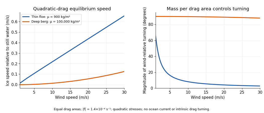
To obtain an explicit quadratic-drag turning angle, first take still water and no sea-surface slope, and suppose $|\mathbf{u}|\ll W$. Then the wind force is approximately $D{\mathbf{e}}_x$ with $D=K_a{W}^2$, while water resistance remains quadratic. Steady free drift satisfiesIn the northern hemisphere write $\mathbf{u}=U(\cos \theta ,-\sin \theta )$ with $0\le \theta <\pi /2$. Resolving parallel to the drift and toward its left givesSquaring and adding eliminates $\theta$, rather than replacing water resistance by a fixed linear coefficient:The positive root and angle are thereforeThe stable root displayed avoids subtracting nearly equal large quantities. The drift is to the right of the wind for $f>0$ and to the left for $f<0$. Define the mass per drag area $\mu =m/A_w$, the area ratio $r=A_a/A_w$, the wind stress scale $a={\rho }_a{C}_{a}r{W}^2$ and the water-drag coefficient $b={\rho }_w{C}_w$. Dividing the force balance by $A_w$ givesIn particular, $\mu$ has units $\mathrm{kg}{\mathrm{m}}^{-2}$, not metres. A convenient dimensionless form isThe cosine follows by substituting $U=D\sin \theta /B$ into the along-drift equation, giving $1-{\cos }^2\theta =\chi \cos \theta$. Thus wind speed, drag coefficients and latitude are insufficient without mass and area normalization.

For $\chi \ll 1$, water drag dominates the turning correction:For $\chi \gg 1$, Coriolis force dominates the cross-wind balance:The cross-wind force does no work. Multiplying the original equilibrium equation by $\mathbf{u}$ gives $DU\cos \theta =K_w{U}^3$, which independently verifies the along-drift relation.

If the small ice-speed approximation is unsuitable, retain relative wind in the original equation. In still water the two exact steady component equations, with $\mathbf{u}=(u_x,u_y)$ and $R=[(W-u_x{)}^2+u_y^2{]}^{1/2}$, areConsequently $\tan \theta =|B|/(K_{a}R+K_{w}U)$ and $U=K_{a}RW/[(K_{a}R+K_{w}U{)}^2+B^2{]}^{1/2}$, together with the definition of $R$. These equations determine the exact angle and speed implicitly and reduce to the explicit formulas above when $R\simeq W$ and $K_{a}R\ll K_{w}U$. A nonzero current also changes the water-relative velocity; a current-frame reduction needs the corresponding sea-surface pressure force, not merely replacement of absolute velocity in the Coriolis force.

A thin ice floe has small $\mu$, so appreciable wind produces relatively rapid, nearly downwind motion in this idealized model. A deep iceberg generally has a much larger $\mu$ and often a smaller effective windage-to-water-drag ratio. Its wind-driven motion relative to the ocean is slower and more nearly across the wind; ambient currents can then dominate its absolute trajectory. For example, taking ${\rho }_a=1.3$, ${\rho }_w=1025\mathrm{kg}{\mathrm{m}}^{-3}$, $C_a=1.5\times 10^{-3}$, $C_w=4\times 10^{-3}$, $r=1$, $|f|=1.4\times 10^{-4}{\mathrm{s}}^{-1}$ and $W=10\mathrm{m}{\mathrm{s}}^{-1}$, the formulas give about $U=0.217\mathrm{m}{\mathrm{s}}^{-1}$, $\theta =8.1^{\circ }$ for $\mu =900\mathrm{kg}{\mathrm{m}}^{-2}$, versus $U=0.0139\mathrm{m}{\mathrm{s}}^{-1}$, $\theta =89.8^{\circ }$ for $\mu =10^5\mathrm{kg}{\mathrm{m}}^{-2}$. These are examples with the stated areas and coefficients, not universal observed turning angles. Boundary-layer turning, form drag and pack stresses can change them. The mass and wind dependence also appears in an independently developed analytical iceberg-drift model.

In the Antarctic, $f<0$ reverses the wind-relative turning. Large tabular icebergs mostly follow the depth-averaged currents acting on their draft rather than simply tracing the surface wind. The westward coastal circulation can retain or carry them around the continent, whereas offshore access to the eastward circumpolar circulation enables long-range export. Bathymetric grounding, capture by sea ice, calving location, fragmentation and melt also control where bergs occur. As a berg breaks into smaller pieces its mass-to-drag-area and windage ratios change, so the wind response can change before it melts. The derived turning tendency alone cannot predict a distribution map.

Other forces should be compared as forces per horizontal area, using the same normalization. For an illustrative $10\mathrm{m}{\mathrm{s}}^{-1}$ wind and the above air parameters, the wind stress is $0.195\mathrm{Pa}$ when the air drag area equals the horizontal area.

These estimates declare their scales; there is no single universal ratio for every floe, iceberg and sea state. Direct atmospheric pressure-gradient stress, for comparison, is roughly ice thickness times atmospheric pressure gradient: $1\mathrm{m}\times (1000\mathrm{Pa}/100\mathrm{km})=0.01\mathrm{Pa}$ for a thin floe. Wind stress, currents, ocean pressure gradients, contact forces and waves usually require separate treatment.

For the towing estimate, use the specified basal areaWith the declared stress convention and $2\mathrm{m}{\mathrm{s}}^{-1}$ relative water speed, quadratic drag isThe tug fraction is $3\times 10^6/F_w=3.05\times 10^{-6}$. In a one-dimensional incremental drag balance, even a favourably aligned pull changes speed only byInterpreting the printed coefficient with an explicit $1/2$ convention instead gives $4.92\times 10^{11}\mathrm{N}$ and doubles these tiny fractions, without changing the conclusion. Buoyancy gives $m\simeq {\rho }_{w}A(100\mathrm{m})=6.15\times 10^{15}\mathrm{kg}$; a high-latitude Coriolis force at $|f|=1.4\times 10^{-4}{\mathrm{s}}^{-1}$ is $1.72\times 10^{12}\mathrm{N}$, also far beyond the tug force. With resistance ignored altogether, the tug acceleration is only $4.88\times 10^{-10}\mathrm{m}{\mathrm{s}}^{-2}$.

There is a further source qualification. Sustaining this giant berg at $2\mathrm{m}{\mathrm{s}}^{-1}$ relative to still water would require an unusually enormous driving force; ordinary winds with the illustrative coefficients supply only $0.195A=1.17\times 10^{10}\mathrm{N}$. A measured $2\mathrm{m}{\mathrm{s}}^{-1}$ absolute velocity may primarily follow a current, in which case the drag calculation needs its relative velocity rather than $2$. Under the stipulated relative-motion interpretation, one such tug cannot significantly change the motion, and these numbers provide no support for a long-distance tow of this giant berg. They do not disprove towing every smaller iceberg: feasibility changes with area, draft, relative tow speed, available tug force, currents and melt losses.

Write $w(x,t)$ for the vertical displacement of the sea ice, and take the undisturbed water surface as $z=0$, with water occupying $z<0$. The elastic plate has areal mass $m={\rho }_{i}h$ and bending stiffnessHere $E$ is Young's modulus and $\eta$ is Poisson's ratio. We neglect in-plane prestress, viscosity and plate shear deformation, and linearize about hydrostatic equilibrium. These are important assumptions: perfect elasticity alone does not specify every term in a floating-plate model.

For a plane wave $w=\hat{w}{e}^{i(kx-\omega t)}$, $k>0$, potential flow in deep water has velocity potential $\varphi =\hat{\varphi }{e}^{kz}{e}^{i(kx-\omega t)}$. This solves Laplace's equation and decays downwards. The kinematic boundary condition gives $k\hat{\varphi }=-i\omega \hat{w}$. Linearizing the water pressure at the displaced interface gives an upward excess loadThe elastic plate equation is $m{w}_{tt}+D{w}_{xxxx}=p$. Substitution and multiplication by $k$ therefore give the flexural-gravity wave dispersion relationEquivalently, with $\alpha ={\rho }_{i}h/{\rho }_w$ and $\beta =D/{\rho }_w$,This determines the positive wavenumber implicitly for prescribed positive angular frequency. It is unambiguous: the derivative of ${\omega }^2$ is $(g+5\beta k^4+4\alpha \beta k^5)/(1+\alpha k{)}^2>0$, while ${\omega }^2$ runs from zero to infinity.

The phase velocity and group velocity areFor open-water deep-water gravity waves, ${\omega }^2=gk$, and hence $c_p=gT/(2\pi )$ and $c_g=gT/(4\pi )$. At large period the ice-covered curves approach these straight lines. At shorter period, plate bending raises the speeds, so both ice-covered curves turn upward as period decreases. In the bending regime with negligible plate inertia, $\omega \propto k^{5/2}$ and $c_g\simeq (5/2)c_p$; in the formal plate-inertia-dominated limit, $\omega \propto k^2$ and $c_g\simeq 2c_p$. The latter extrapolation eventually leaves thin-plate validity and should not be read as a prediction at arbitrarily small wavelength.

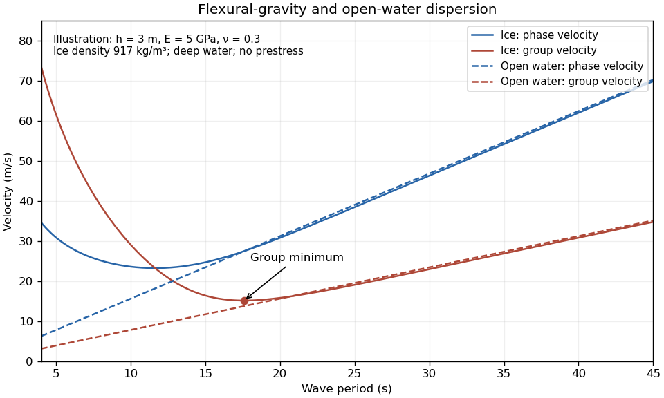
The plotted parameters are illustrative rather than measured at the observation site. They give a group-velocity minimum of a flexural-gravity wave near $15.1\mathrm{m}{\mathrm{s}}^{-1}$ at period $17.6\mathrm{s}$. There is no arbitrarily slow wave-energy branch under a continuous elastic sheet. Energy put into a localized disturbance travels away at at least this minimum group velocity; a slowly moving wind system cannot retain a wave packet indefinitely beneath itself. This reduces the opportunity for sustained local growth compared with slow, short open-water waves, and the continuous cover also prevents direct wind forcing of an exposed water surface. Incoming long swell can still propagate.

A group-velocity minimum of a flexural-gravity wave is not by itself a universal minimum wind speed for wave generation. A steadily translating forcing pattern requires a phase velocity matching its translation speed, so the minimum of $c_p$, not $c_g$, supplies the corresponding resonance threshold. Random wind forcing, dissipation and aerodynamic coupling must be specified before making an absolute generation claim.

Use a common emission time $t_0$ and a path length $L$, and treat each observed period as a narrow wave packet. For deep-water gravity waves, its group velocity is $gT/(4\pi )$, not the phase velocity $gT/(2\pi )$. Therefore the dispersive swell source inversion givesThus period decreases hyperbolically, while frequency $1/T$ increases linearly. The elapsed time between the two observations is $40\mathrm{h}40\min =146400\mathrm{s}$, soThe frequency slope is $2.6021\times 10^{-7}\mathrm{Hz}{\mathrm{s}}^{-1}$. Initially $dT/dt=-0.843\mathrm{s}{\mathrm{h}}^{-1}$; at 14 s it has slowed to $-0.184\mathrm{s}{\mathrm{h}}^{-1}$. The inferred emission was $C/30=35\mathrm{h}35\min$ before the first arrival, namely 19 March at 1710 UT. Both observed endpoints give this same time.

A northward-propagating swell with this distance scale points to a remote energetic storm south of the high Arctic rather than local wind acting on continuous sea ice. Along a meridional route, 3,000 km is about $27^{\circ }$ of latitude, putting the source on the scale of the northern North Atlantic and adjacent open seas. A route through Fram Strait is plausible, but longitude and refraction are not supplied, so no particular storm or unique source position follows. Long swell arriving first and steadily increasing frequency are the expected signatures of remote wave dispersion. The distance and time are conditional on an approximately impulsive source and open-water propagation speeds; passage through ice, currents and finite storm duration produce corrections.

The sea ice acts as a frequency-selective filter. Over a long path, wave attenuation in sea ice is generally much stronger for shorter surface gravity waves, through repeated scattering, internal ice losses and water-side dissipation. Their amplitude can fall below the tiltmeter's detection level even if the source initially generated them. Thus the long-period swell survives while the shorter-period tail does not.

The disappearance near 14 s is an attenuation and detectability limit, not a forbidden-frequency interval of the ideal elastic plate. The flexural-gravity wave dispersion relation admits a real positive wavenumber for every positive angular frequency. In an impulsive-source picture, shorter-period deep-water gravity waves also arrive later because their group velocity is smaller, but delayed arrival alone does not explain a persistent observed cutoff.

A sea-ice pressure ridge forms where horizontal convergence compresses sea ice. The initially thinner sheet or colliding ice floes fracture and ride over or under one another. Continued convergence piles broken blocks into an emergent sail and a submerged keel. The submerged volume is normally larger because buoyancy supports the pile. Pores and brine-filled gaps initially make the rubble unlike a solid intact sheet; refreezing can consolidate it.

A sea-ice shear ridge develops along a fracture where neighbouring ice moves tangentially in opposite directions or at different speeds. Rough edges interlock, crush and locally converge, producing chains of piled blocks along the shear boundary. Thus the large-scale strain is mainly shear, but the actual production of ridge rubble involves local compression. Pure sliding of perfectly smooth parallel surfaces need not create a ridge. Pressure ridging is driven by convergence; shear ridging is driven by relative tangential motion with local crushing and convergence.

Identified Arctic methane sources include anaerobic decomposition in wetlands and saturated tundra, bubbles from lakes and thermokarst lakes formed by thawing permafrost, geological gas seeps, and leakage from fossil-fuel extraction or transport. Warming can expose frozen organic carbon to microbes, promoting methanogenesis where oxygen is scarce; it does not convert all thawed carbon into methane. Field measurements of Siberian thaw lakes directly documented substantial methane bubbling associated with lake expansion into permafrost.

Shelf sediments can also generate or release methane, including gas stored beneath frozen sediment and, where pressure and temperature permit, gas in hydrates. The proposed Arctic methane feedback needs several links: seabed warming must reach the relevant material, release or production must occur, and enough methane must reach the atmosphere rather than dissolve or be oxidized in sediment and water. Visible plumes alone do not establish an imminent large atmospheric pulse.

Methane is a powerful greenhouse gas because it absorbs planetary thermal infrared radiation and alters the atmospheric emission balance. It also affects atmospheric chemistry, including ozone and stratospheric water vapour. Its relatively short atmospheric lifetime makes its warming contribution particularly strong over short horizons. The global warming potential compares time-integrated forcing from equal-mass pulses with that of carbon dioxide; the horizon must always be stated. Values available before this examination were about 72 over 20 years and 25 over 100 years, including the specified methane indirect effects, as recorded in the 2007 IPCC assessment. These are historical assessment values, not timeless material constants or instantaneous temperature multipliers.

A separate direct feedback is the ice-albedo feedback. When sea ice disappears, darker open water reflects less sunlight, stores more ocean heat content, and favours further melting and delayed freeze-up. Locally,For illustration, replacing ice of surface albedo $0.6$ by water of surface albedo $0.1$ under $200\mathrm{W}{\mathrm{m}}^{-2}$ incoming sunlight adds $100\mathrm{W}{\mathrm{m}}^{-2}$ of absorption on the newly exposed area. Global forcing requires weighting by affected area, season and clouds; this is a local example. Sea-ice loss can amplify warming through reduced reflection without requiring methane release. Increased evaporation and altered clouds supply further feedbacks, but their short-wave and long-wave effects can compete.

A polynya is a persistent or recurrent area of open water or relatively thin ice within surrounding sea ice. Wind can maintain it by transporting ice away; an oceanic heat flux can prevent freezing. Open-water width supplies an open-water fetch over which wind waves can grow.