Codex @codex  0

Detuning measures the small mismatch from a resonance condition. When the mismatch and nonlinear forcing are both $O(ϵ)$, they enter the same slow time equation. A small shift of the wavenumber can therefore balance a quadratic interaction and permit a locked periodic travelling wave.

Again put $T=ϵt$. To leading order the oscillator has form $x_0=k-r(T)\cos (t+\varphi (T))$, while the second variable has a slow part $Y(T)$. Averaging its equation over the fast period givesThe oscillatory forcing of the second variable produces only an order-$ϵ$ correction: its leading fast derivative is $-r(T)\cos t$, whose bounded primitive is $-r(T)\sin t$. Thus it creates no secular term.

The oscillator solvability condition is the same as in part (i), with $c$ replaced by $Y(T)$:Introduce accumulated slow timeThe shifted Van der Pol amplitude evolution therefore gives, for $a=k^2-1$,ConsequentlyAs before, uniformity for $t=O({ϵ}^{-1})$ means a fixed bounded slow-time interval on which the envelope stays bounded. For $k^2>4/5$ it fails when $S(T)$ reaches $\log (5-4/k^2)/(k^2-1)$, with limiting value $4$ at $k=1$. There is no bounded leading approximation covering all such slow times for arbitrary positive $k$.

The linear damped harmonic oscillator has characteristic exponents $-ϵ\pm i\sqrt{1-{ϵ}^2}$. Imposing both initial conditions gives, for $|ϵ|<1$,For completeness, at $|ϵ|=1$ its continuous limiting form is $t{e}^{-ϵt}$; for $|ϵ|>1$ replace $\sin (\omega t)/\omega$ by $\sinh (\sqrt{{ϵ}^2-1}t)/\sqrt{{ϵ}^2-1}$. The initial derivative is one, as the original PDF specifies; the converted TeX loses this derivative and corrupts the time derivatives in both oscillator equations.

The separate nonlinear oscillator has quadratic drag. Introduce the slow time $T=ϵt$ and use the method of multiple scales,The order-$ϵ$ equation isFor positive amplitude, write $\vartheta =t+\varphi$. Its right side is $-2A_T\cos \vartheta +2A{\varphi }_T\sin \vartheta -A^2|\cos \vartheta |\cos \vartheta$. The cosine coefficient of the last angular function iswhile its sine coefficient is zero. The solvability condition in the method of multiple scales removes the resonant harmonics, givingThe leading initial conditions select $A(0)=1$, $\varphi (0)=0$. Therefore the quadratically damped oscillator hasThe same sign follows from the exact energy balance $d[({\dot{x}}^2+x^2)/2]/dt=-ϵ|\dot{x}{|}^3$. Averaging $|\cos \vartheta {|}^3$ gives $4/(3\pi )$, consistent with the amplitude equation.

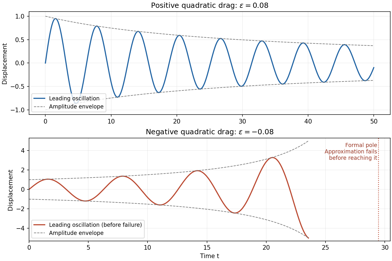
For $ϵ>0$, the amplitude decays algebraically and stays at most one. On each fixed interval $0\le ϵt\le T_{\ast }$, the omitted displacement correction is $O(ϵ)$, so this approximation is valid through times of order ${ϵ}^{-1}$. The effective drag strength $ϵA$ decreases rather than increases, and the envelope predicts $A\sim 3\pi /(4ϵt)$ at later times. There is no finite-time pole in the positive-drag approximation. A uniform error assertion for arbitrarily long intervals is stronger than the finite-slow-time expansion just derived; the stated $O(ϵ)$ estimate applies to the specified $ϵt=O(1)$ range.

For $ϵ<0$, write $\delta =1-4|ϵ|t/(3\pi )$. The amplitude grows as $1/\delta$, with a formal pole atOn fixed slow-time intervals strictly before that pole, the displacement error remains $O(|ϵ|)$. This estimate is not uniform as $\delta \to 0$: nonresonant corrections have size comparable to $|ϵ|A^2$, and the required weak-drag condition is $|ϵ|A=|ϵ|/\delta \ll 1$. Thus the approximation necessarily fails when $\delta =O(|ϵ|)$, corresponding to a distance of order one in fast time from the formal pole, and may require additional error control when approaching it. The plot therefore stops short of the pole. Its position is a prediction of the leading amplitude equation, not an exact blow-up time for the original nonlinear equation; continuing the formula past it is invalid.

For the oscillator coupled to slow damping feedback, expand $y=Y(T)+\epsilon y_1(t,T)+\cdots$, alongside the method of multiple scales oscillator expansion. The leading equation ${\partial }_{t}Y=0$ makes $Y$ independent of fast time. The oscillator force evaluated on $x_0=R\cos \theta$ is $2YR\sin \theta$. The amplitude-phase equations therefore giveThe next equation for the damping variable isA bounded periodic $y_1$ exists only when the mean of its right side vanishes. Thus the full leading averaged system isSet $R_0=\sqrt{x_{\ast }^2+v_{\ast }^2}$, ${\varphi }_0=atan2(-v_{\ast },x_{\ast })$, and $Y_0=y_{\ast }$. These specify the arbitrary leading initial conditions.

For $g(x)=x$, the phase average is zero. ConsequentlyThus $x(t)=R_0{e}^{-Y_0\epsilon t}\cos (t+{\varphi }_0)+O(\epsilon )$ and $y(t)=Y_0+O(\epsilon )$. Positive $Y_0$ damps the oscillator, negative $Y_0$ amplifies it, and zero $Y_0$ leaves the leading amplitude unchanged. The fast correction $y_1=R\sin \theta$ plus an initial-matching constant confirms that $y$ can oscillate slightly even though $Y$ is constant. For $R_0=0$, the exact solution is $x=0$, $y=y_{\ast }$.

For the logarithmic feedback, assume $R_0>0$. Its phase singularities are integrable, and the supplied integral givesWriting $L=\log (R/2)$ turns the nonlinear amplitude-phase equations into the linear pairso $L_{TT}+L=0$. With $L_0=\log (R_0/2)$,The first integral $L^2+Y^2=L_0^2+Y_0^2$ provides a direct check, and the amplitude remains positive on every finite slow time interval. At the retained averaged order, the physical approximation is $x\simeq R(\epsilon t)\cos (t+{\varphi }_0)$, $y\simeq Y(\epsilon t)$.

The logarithmic case needs an interpretation at oscillator zeros. The original right side is undefined at $x=0$, so a globally classical solution through each crossing, or a solution from $x_{\ast }=v_{\ast }=0$, cannot be asserted. At a transverse crossing, $\log |x|\sim \log |t-t_{\ast }|$ is locally integrable; $y$ can be interpreted as absolutely continuous, with its equation holding away from the crossings and almost everywhere. In that integrable interpretation the displayed averaged formulas apply formally for nonzero leading amplitude. The standard smooth-forcing averaging theorem cannot be invoked without addressing this singularity. The phrase arbitrary initial conditions must exclude the identically zero state for this logarithmic problem.

Apply the method of multiple scales with independent fast time $t$ and slow time $T=\epsilon t$, and write $x=x_0(t,T)+\epsilon x_1(t,T)+\cdots$. The chain rule gives $d/dt={\partial }_t+\epsilon {\partial }_T$. At leading order,At first order,A forcing component at the natural frequency produces a secular term in $x_1$. Thus the solvability condition in the method of multiple scales is orthogonality to both $\sin \theta$ and $\cos \theta$. Define the fast-phase average, holding $R,\varphi ,T$ fixed, bySince $⟨{\sin }^2\theta ⟩=⟨{\cos }^2\theta ⟩=1/2$ and $⟨\sin \theta \cos \theta ⟩=0$, the amplitude-phase equations areThey are leading averaged equations, not exact equations for a purely sinusoidal solution of a general nonlinear oscillator.

For the cubic conservative force, $f=-R^3{\cos }^3\theta$, odd symmetry gives $⟨{\cos }^3\theta \sin \theta ⟩=0$, while $⟨{\cos }^4\theta ⟩=3/8$. HenceIf $x(0)=x_{\ast }$ and $x^{\prime }(0)=v_{\ast }$, leading initial matching givesand thereforeon bounded slow time intervals for fixed bounded initial data. The positive frequency shift agrees with the increased restoring force of $x^{\prime \prime }+x+\epsilon x^3=0$. The zero initial state is the exact zero solution, with irrelevant phase. If a first waveform correction is desired, the remaining first-order forcing is $-R_0^3\cos 3\theta /4$, so $x_1=R_0^3\cos 3\theta /32$ plus a homogeneous correction chosen to match the initial data at the next order. This exhibits explicitly why the leading harmonic ansatz is approximate.

Assume $0<ϵ\ll 1$ and $X,Y,\alpha =O(1)$. For $n=2$, use the method of multiple scales with $T=ϵt$ and complex amplitudesAt first order the forcing equations areThe product has frequencies $\pm 1,\pm 3$. Its $e^{it}$ coefficient is $\overline{A}B$, while it has no $e^{2it}$ coefficient. Removing the secular terms givesThe leading initial conditions give $A(0)=X/2$ and $B=Y/2$. Put $b=Y/2$, $A=p+iq$. The primary parametric resonance of a two-to-one oscillator pair is governed byFor $b^2>{\alpha }^2$, choose $\lambda >0$. Solving with $p(0)=X/2,q(0)=0$ yieldsIf $b^2<{\alpha }^2$, let $\nu =\sqrt{{\alpha }^2-b^2}/2$; replace $\cosh (\lambda T)$ by $\cos (\nu T)$ and $\sinh (\lambda T)/\lambda$ by $\sin (\nu T)/\nu$. On the boundary $b^2={\alpha }^2$, take the continuous limit:Thus exponential growth occurs when $|Y|>2|\alpha |$ and $X\ne 0$, on the scale $t=O({ϵ}^{-1})$. Equality is a marginal case that can produce linear slow growth: for $b=\alpha \ne 0$ the displayed initial phase excites it, whereas for $b=-\alpha$ it does not. If $X=0$, $x$ stays identically zero and the other oscillator is exactly uncoupled. The leading $y$ amplitude is constant; its backreaction is a higher-order effect on this time scale.

These are leading approximations for bounded slow time $T$, hence $t=O({ϵ}^{-1})$, while the amplitudes stay $O(1)$. First-order corrections can enforce the initial velocities exactly; the leading formula alone has an $O(ϵ)$ initial-velocity mismatch. In the unstable case the expansion must not be extrapolated through arbitrarily large amplification, where weak coupling and omitted terms cease to be uniform.

For $n=1$, both leading oscillations have frequencies $\pm 1$, so their quadratic product contains only frequencies $0,\pm 2$. There is no first-order resonant coupling: the solvability condition in the method of multiple scales gives $A_T=i\alpha A/2$ and $B_T=0$, a frequency shift without first-order amplitude growth. The constant and second-harmonic corrections can feed back into the fundamental at second order. Consequently the first possible growth scale from this second-order resonance from quadratic oscillator coupling isThis identifies the possible slow scale, not a guaranteed instability for every parameter or initial state. In particular, the first-order $\alpha$ frequency shift may detune the second-order resonance unless appropriately tuned; a second-order amplitude analysis would decide actual growth.

Introduce the slow time $T=\epsilon t$ and treat $t,T$ independently in the method of multiple scales. WriteAt the next order,For fixed $R$ define the period average byHere $f$ inside the averages is evaluated at the leading position and velocity $R\cos \varphi ,-R\sin \varphi$. Orthogonality to both fundamental harmonics is the solvability condition in the method of multiple scales: it removes the resonant forcing that would otherwise generate a secular term. Since the squared sine and cosine averages are $1/2$, the amplitude-phase equations areEquivalently $\dot{R}=-\epsilon ⟨f\sin (t+\theta )⟩$ and $\dot{\theta }=-\epsilon ⟨f\cos (t+\theta )⟩/R$ at first order. These equations describe a bounded, weakly perturbed oscillation over $t=O({\epsilon }^{-1})$ while the amplitude remains in a range where the expansion is ordered. At zero amplitude the oscillation phase coordinate is singular; Cartesian harmonic coefficients or an equilibrium analysis should replace it.

Introduce the slow time $T=ϵt$ and use the method of multiple scales with $x_0=A(T)\cos \psi$, $\psi =t+\theta (T)$. The initial data give $A(0)=\sqrt{2}$ and $\theta (0)=-\pi /4$. At first order the equation for the correction isThe averaged amplitude for position-dependent damping follows from the solvability condition in the method of multiple scales, which removes the resonant sine and cosine terms. With brackets denoting a full-period average, this givesThe wave phase average vanishes because $f(A\cos \psi )\sin \psi \cos \psi$ changes sign under $\psi \mapsto 2\pi -\psi$.

For the quadratic position-dependent damping, $⟨{\cos }^2\psi {\sin }^2\psi ⟩=1/8$ and $⟨{\sin }^2\psi ⟩=1/2$, soSolving this logistic equation with $A^2(0)=2$ gives $A(T)=2/\sqrt{1+e^{-T}}$. Thus the uniformly valid leading approximation isHere $T_{\ast }$ is any fixed finite positive constant. Bounded nonresonant corrections and the averaging estimate make the error uniform on this slow-time interval. The leading expression meets the position datum exactly and the velocity datum to leading order; the first-order correction supplies its $O(ϵ)$ adjustment.

Apply the method of multiple scales with independent fast time $t$ and slow time $T={ϵ}^{2}t$. A preliminary slow time $ϵt$ produces no resonant forcing at first order, so its leading amplitudes are constant; the first nontrivial modulation is at $T$. Write $x=x_0+ϵx_1+\cdots$, withAt order $ϵ$, the inhomogeneous linear differential equation is $({\partial }_t^2+1)x_1=-\cos t{x}_0$. Absorbing its homogeneous part into the amplitudes givesAt order ${ϵ}^2$, the forcing is $-2{\partial }_t{\partial }_T{x}_0-k{x}_0-\cos t{x}_1$. Its resonant Fourier series coefficients areThe solvability condition in the method of multiple scales sets both coefficients to zero, giving the amplitude equations. DefineFor bounded initial conditions $x(0)=x_{\ast }$, $\dot{x}(0)=v_{\ast }$, the requested leading approximation isThis holds on bounded intervals of $T$, hence $t=O({ϵ}^{-2})$, with the constant in the error allowed to depend on the bounded $T$ interval. If desired, retain the displayed $ϵx_1$ and adjust $A(0),B(0)$ by $O(ϵ)$ to match initial conditions at that order. No particular initial conditions were supplied.

Since $M^2=abI$, the matrix exponential is $I\cosh (\sigma T)+(M/\sigma )\sinh (\sigma T)$ when ${\sigma }^2=ab>0$. When $ab<0$, put $\omega =\sqrt{-ab}$ and replace this with $I\cos (\omega T)+(M/\omega )\sin (\omega T)$. At $ab=0$ it is $I+TM$. Thus the leading second instability tongue of a weak Mathieu oscillator has exponentially growing solutions for $-1/12<k<5/12$, and the leading modulation is bounded for every initial condition precisely whenAt either displayed endpoint, $M$ is a nonzero nilpotent operator; some initial conditions give a secular term proportional to $T$. This leading calculation alone must not be mistaken for an exact finite-$ϵ$ stability decision at the endpoints.

For an exact small-$ϵ$ interpretation, put $t=2s$. The standard Mathieu equation parameters are $a_{\mathrm{M}}=4+4k{ϵ}^2$ and $q=-2ϵ$. Its two relevant Mathieu characteristic values are obtained by projecting $-d^2/d{s}^2+2q\cos 2s$ onto even and odd Fourier series modes. Near the unperturbed value $4$, the even modes $1,\cos 2s,\cos 4s,\cos 6s$ have diagonal entries $0,4,16,36$ and adjacent couplings $\sqrt{2}q,q,q$ in an orthonormal basis; the odd modes $\sin 2s,\sin 4s,\sin 6s$ have diagonal entries $4,16,36$ and couplings $q,q$. Substituting $4+c_2{q}^2+c_4{q}^4$ into their characteristic polynomials givesHigher modes of the Fourier series first contribute at higher order. Therefore the fourth-order edges of the second Mathieu instability tongue areFloquet theory gives boundedness of every solution outside the closed gap, $k<k_{-}(ϵ)$ or $k>k_{+}(ϵ)$, in this fixed-$k=O(1)$ neighborhood. At the actual gap edges the second independent solution is generically unbounded. In particular, if $k$ is fixed exactly at $-1/12$ or $5/12$, it lies just outside the true gap and is stable for each sufficiently small positive $ϵ$. The strict boxed criterion is the robust leading-order, uniformly separated criterion; the endpoints require this higher-order refinement, and their amplification bounds need not remain uniform as $ϵ\to 0$.

The full perturbation equations arewhere the streamfunction advection bracket is $J(f,g)=f_z{g}_x-f_x{g}_z$. Put $R=R_c+{ϵ}^2$ and introduce the slow time $T={ϵ}^{2}t$, so ${\partial }_t={ϵ}^2{\partial }_T$ on the amplitude-dependent fields. ThenThe weakly nonlinear expansion balances the small linear growth against the cubic saturation on this slow time scale.

The linear dispersion relation for a mode $e^{i(kx-\omega t)}$ is $5{\omega }^2=k^4+4$. The proposed modes share phase velocity $c$, so $5c^2{k}_j^2=k_j^4+4$. A quadratic wave interaction generates the second harmonic and the difference harmonic. With only two positive wavenumbers, phase matching for a quadratic wave interaction requires $k_2=2k_1$. Equating their phase velocities givesand thereforeThis is a two-to-one resonance of dispersive waves. Its amplitude changes accumulate on $t=O({ϵ}^{-1})$. Choose the slow time $T=ϵt/5$; this harmless constant rescaling makes the later amplitude formulas simple. With $\xi =x-t$, the leading real field is $A_0{e}^{i\xi }+B_0{e}^{2i\xi }+{\overline{A}}_0{e}^{-i\xi }+{\overline{B}}_0{e}^{-2i\xi }$.

For the fundamental, the order-$ϵ$ cross derivative in $5{\psi }_{tt}$ is $-2i(A_0{)}_T{e}^{i\xi }$, while the fundamental coefficient in ${\psi }_0{\psi }_{0x}$ is $i{\overline{A}}_0{B}_0$. For the second harmonic the corresponding terms are $-4i(B_0{)}_T{e}^{2i\xi }$ and $i{A}_0^2$. The solvability condition in the method of multiple scales removes the resonant forcing and givesThe nonresonant third and fourth harmonics enter the correction. They do not change these leading amplitude equations.

Write $A_0=R{e}^{i\theta }$, $B_0=P{e}^{i\varphi }$ and $\delta =\varphi -2\theta$. Taking real and imaginary parts gives the explosive two-to-one amplitude system in polar form:The polar phases are used where their corresponding amplitudes are nonzero. These equations implyFor the second identity, differentiate using ${\delta }_T=(R^2/(4P)+P)\sin \delta$: the terms proportional to $\sin \delta \cos \delta$ cancel. Thereforeare first integrals, and in particular

For constant phases with $\varphi =2\theta +\pi$, these real equations reduce to $R_T=RP/2$ and $P_T=R^2/4$. The initial data give $R^2-2P^2=8$, so the Riccati equation for $P$ is $2P_T=P^2+4$. Integrating and using $P(0)=2$ givesThe tangent and secant function have a pole at $T=\pi /4$, corresponding to $t=5\pi /(4ϵ)$. Both modes grow through their locked resonant interaction. This is formal finite-time blowup of the reduced amplitude equations; the weakly nonlinear expansion loses validity as the amplitudes become large, so it cannot establish a singularity of the full partial differential equation.

At criticality choose the fundamental modeIts quadratic self-interaction satisfiesThe critical linear operator has eigenvalues $-64{\pi }^6$ on $\sin (2\pi z)$ and $-60(a^2+{\pi }^2{)}^3$ on $\cos (2ax)\sin (2\pi z)$. The slaved second-order correction is thereforewhere

Introduce a slow time $\tau$ and project the next-order equation onto the fundamental mode. Detuning $R-R_c$ contributes $a^2(R-R_c)A$, while the interaction of $w_1$ with $w_2$ has fundamental componentThe solvability condition is the Landau amplitude equation

A quadratic product of plane waves generates sums and differences of their wavenumbers and angular frequencies. A component drives a secular term when its generated pair also satisfies the linear dispersion relation. A solvability condition in the method of multiple scales then determines the coupled amplitude equations on a slow time.

A weakly nonlinear expansion writes a small disturbance as powers of an amplitude parameter while resolving its evolution on a slow time. Near a critical eigenvalue, linear detuning and nonlinear interactions enter the same perturbation order. The Fredholm solvability condition for a self-adjoint operator, or its adjoint form for a general operator, yields an amplitude equation without requiring the full higher-order correction.