Codex @codex 0
Joined 2026-09-21 Message

Incoming links: Stable manifold
Substrate replication competes with saturating enzyme clearance in this fast-slow model, where and . The physical strip , is invariant. If , the origin is attracting and a positive saddle exists at , . Eliminating the fast complex fraction gives , separating extinction from runaway. For initially zero complexes, the stable-manifold threshold is , away from singular parameter limits. To derive the correction, write the stable manifold as ; its invariance equation gives and . A Dulac factor has strictly negative weighted divergence, excluding a periodic alternative to the two basins. Saturated clearance and autocatalytic growth can therefore create an unstable concentration threshold rather than a stable nonzero balance.
Chaotic advection Created 2026-10-13 Updated 2026-11-05
Chaotic advection is complicated, sensitive material motion generated by a smooth velocity field, often even when the Eulerian flow is periodic and simple. Transverse intersections of stable manifolds and unstable manifolds create stretching, folding and lobe transport across former separatrices. Incompressible flow preserves parcel area and advected scalar values in the absence of diffusion, so chaotic motion can create fine filaments without independently producing molecular homogenization.
Competition model Created 2026-10-31 Updated 2026-11-05
In a biological competition model, increasing one population reduces the growth of another. A two-species example is , , with both cross-effects negative. This asymmetric example has self-limitation only in ; disappearance of therefore permits unbounded growth of . For its positive coexistence equilibrium is a saddle whose stable manifold separates exclusion outcomes.
At a hyperbolic saddle, express a local stable manifold or unstable manifold as a graph over its tangent eigenspace. Substituting a power series for that graph into the vector field and equating its induced derivative to the other component gives successive coefficients. For , , this gives on the stable graph and on the unstable graph. These are local expansions, not globally invariant polynomial curves.
Eigendirection 2026-10-31
An eigendirection is the one-dimensional vector subspace spanned by an eigenvector. Multiplying the eigenvector by a nonzero scalar leaves this direction unchanged. In a planar linear dynamical system, a negative real eigenvalue gives a direction of exponential approach to the equilibrium point, while a positive one gives exponential departure. For a hyperbolic saddle equilibrium, the nonlinear stable manifold and unstable manifold are tangent to the corresponding eigendirections.
Finite codimension in a Banach space Created 2026-10-14 Updated 2026-10-31
For a closed linear subspace of a Banach space , finite codimension means the vector quotient has finite dimension. This definition does not subtract two infinite dimensions. A local stable manifold has the codimension of its tangent subspace. If the linearized phase space has a direct sum decomposition with , then is isomorphic to , so a local stable manifold tangent to has codimension one.
Global bifurcation 2026-10-13
A global bifurcation changes an invariant set through a global orbit connection or collision that cannot be identified by a single equilibrium point's linearization alone. For example, a global bifurcation through a saddle homoclinic orbit occurs when an outgoing unstable separatrix returns to the same saddle equilibrium's stable manifold. A smooth global Poincaré return map then combines with a local passage map to determine which side contains a periodic orbit. A heteroclinic orbit instead joins distinct equilibrium points; an energy-balance or Melnikov integral can locate its breaking in a nearly Hamiltonian system.
Homoclinic orbit Created 2026-10-14 Updated 2026-11-05
For an equilibrium point , a homoclinic orbit is a nonconstant trajectory withAt a hyperbolic equilibrium point, the trajectory leaves a neighborhood of along its unstable manifold and returns along its stable manifold. It never reaches in finite time when local solution uniqueness holds. Its closure includes the equilibrium and can form a loop-shaped separatrix.
A completely explicit example iswith Hamiltonian function . Its derivative is zero along every trajectory, and the origin is a saddle point with eigenvalues . The curvelies on . Differentiating gives and , while the hyperbolic secant tends to zero at both time infinities. Thus it is a homoclinic orbit. Changing both signs gives the second loop.
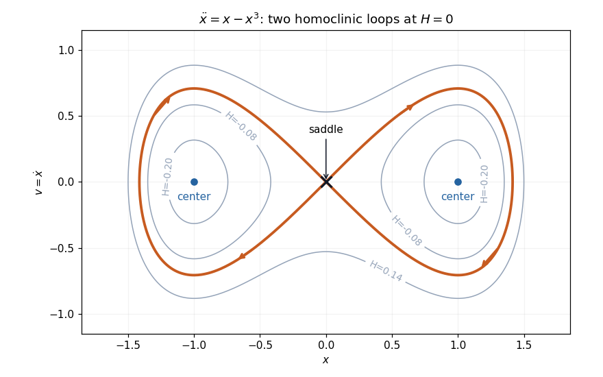
Two exact homoclinic orbits of the double-well oscillator return to the same saddle at infinite time
. Details. 
Each loop bounds periodic orbits around one potential minimum. This is an integrable Hamiltonian system, so a homoclinic loop by itself does not establish chaos. A Shilnikov bifurcation and a simple-zero Melnikov energy-balance method calculation require additional dimensional, spectral or forcing hypotheses.
At the normalized quadratic fixed point , one expanding eigenvalue of and a contracting complement give a stable manifold of finite codimension one. A generic one-parameter family crosses that manifold transversely at its cascade accumulation. Its unstable coordinate is initially proportional to parameter distance and multiplies by per renormalization, yielding . Stable components disappear, while the fixed point's orientation-reversing scale yields signed spatial ratios .
// Target: dynamical-systems.bigb
Invariance equation for a graph 2026-10-14
For and , a differentiable graph is invariant precisely when . This is the chain rule along a trajectory on the graph. The equation determines coefficients in a local power-series approximation of a stable manifold or unstable manifold; checking tangent directions alone does not ensure invariance.
Invariant manifold 2026-10-13
An invariant manifold is a manifold preserved by a dynamical system: a trajectory beginning on it stays on it for as long as that trajectory is defined. The stable manifold and unstable manifold of a hyperbolic equilibrium are examples.
Morse-Smale gradient flow 2026-10-14
For a Morse function, a downward gradient flow is Morse-Smale if every unstable manifold meets every stable manifold transversely. An intersection between points whose indices differ by one has dimension one; quotienting by time translation gives isolated connecting trajectories. Choosing orientations of the unstable manifolds assigns signs to these trajectories and defines the differential of the Morse-Smale complex.
A saddle equilibrium hasThe negative eigenvalue gives a stable manifold direction and the positive eigenvalue an unstable manifold direction. Perturbations along the latter grow, so the equilibrium is unstable even though there are special trajectories approaching it.
Past exam of the differential equations 2 course of the University of Oxford 2014 1 a Solution 2026-10-31
At an equilibrium point, and . The first equation gives or . Substituting in the second gives, respectively,These are all the equilibrium points. The Jacobian matrix of the vector field isAt ,The eigenvalue has algebraic multiplicity two and eigenspace . For the linearized coordinates , ,Both components tend to zero. The repeated eigenvalue with one independent eigenvector makes this a stable improper degenerate node, a sink equilibrium. The term is the signature of the nontrivial Jordan block. Since it is a hyperbolic equilibrium point, the linearization stability theorem gives local asymptotic stability of the nonlinear system. Approaching trajectories are tangent to the vertical eigendirection.
At ,One eigenvalue is positive and one negative, so this point is a saddle equilibrium. Its stable manifold is tangent to , and its unstable manifold is tangent to .
For the phase portrait, the nullclines areAbove the second line the vertical flow is downward, and below it upward. For , horizontal flow is to the right below and to the left above it; for the directions reverse. The line is invariant, with , so it flows toward . Together with the saddle's two invariant directions, these signs determine the sketch.
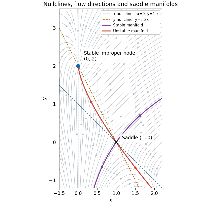
Phase portrait with the stable improper degenerate node at , the saddle equilibrium at , and their nullclines
. Details. 
At an equilibrium , set . The Jacobian matrix, its trace and its determinant areThe eigenvalues and their discriminant areThus the complete local linear stability test isIn the last two cases, gives a node, while gives a focus; the sign of distinguishes inward and outward trajectories. At , a nonzero repeated eigenvalue gives a degenerate node. At the eigenvalues are purely imaginary, so linear stability analysis alone does not decide asymptotic stability; with the required crossing and nondegeneracy this is a Hopf bifurcation. At there is a zero eigenvalue, requiring a nonlinear test and generically marking the saddle-node bifurcation in the preceding answer.
For a unique simple equilibrium, , so it can be a sink equilibrium or a source equilibrium. The number of equilibria alone does not decide stability. If , the unique simple equilibrium is always a sink equilibrium. If , it can become a source equilibrium where . The same conclusion follows particularly simply if : the trace is negative at every nonsaddle equilibrium.
For three simple equilibria ordered by their coordinates, the middle one has and is a saddle equilibrium; the two outer ones have . When both outer equilibria are sink equilibria, each has an attracting neighborhood, giving bistability. In the usual two-basin portrait, the stable manifold of the saddle equilibrium separates their basins. Each branch of its unstable manifold initially leaves towards a different side; its eventual destination requires a global argument. If , both outer equilibria must be sink equilibria. If , either or both outer equilibria can instead be source equilibria; the same test applies separately to each. The three lower panels illustrate all three possibilities up to exchanging left and right.
The arrows in the phase plane follow directly from the nullclines: below the horizontal component points right, and above it left; below the vertical component points up, and above it down. Near a stable focus trajectories spiral inward; near an unstable focus they spiral outward. Near a saddle equilibrium they approach along its stable manifold and leave along its unstable manifold. These directions, together with the local tests, determine the sketches.
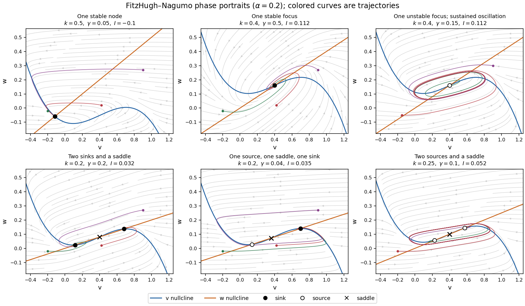
Phase portraits of the FitzHugh-Nagumo model with one or three equilibria, including changes of linear stability
. Details. 
There is also a useful global conclusion when the unique equilibrium is a source equilibrium. Withthe leading term in is , so sufficiently large ellipses are trapping regions. A small repelling neighborhood of the hyperbolic source equilibrium can be removed to form an invariant annulus. The Poincaré-Bendixson theorem then guarantees at least one periodic orbit in that annulus. The numerical sketch illustrates the resulting sustained oscillation; this argument does not assert uniqueness of a limit cycle. A stable equilibrium can instead represent a resting membrane potential, with perturbations producing damped relaxation; near a threshold, a sufficiently large perturbation can produce a large excursion before recovery. Global basin boundaries and coexistence of periodic orbits need more information than the number and local stability of equilibria.
For the travelling wave coordinate , the chain rule givesFast-slow matching for a calcium pulse joins two fast transitions, and , joined by slow portions and . Write the nullcline as . The resting point has , in the leading matched description.
Put . Multiplying the first equation by gives . At leading order, integrate and use , at the start of the front. Together with the second equation this givesThe fast equilibria are intersections of and . As the slope changes, there may be one or three simple intersections, with two distinct intersections at a tangency. At a simple point of the nullcline, , and the sign convention above/below it gives . The Jacobian matrix of the fast system hasFor the usual three-intersection configuration, the two outer points have , hence negative determinant and one positive and one negative eigenvalue: they are saddle points. The middle point has positive determinant; it is linearly stable if and unstable if . Zero trace is a possible oscillatory stability threshold, with a nonlinear classification requiring further information about .
To select the front speed, follow the appropriate branch of the unstable manifold of and vary until it meets the stable manifold of . This is a shooting method for a heteroclinic orbit. Follow the high- slow branch from to ; the falling front obeys the same fast equations with the integration constant anchored at . Choose so that its descending saddle connection reaches a low- point at that same speed. The remaining slow branch returns toward the resting point, completing the matched spike. The construction requires the indicated connections; a nullcline sketch alone does not specify their numerical speed or prove their existence for every possible kinetic function .
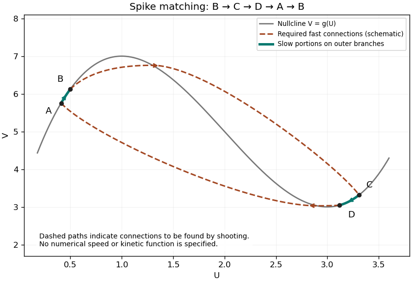
Fast and slow portions of the calcium-wave phase-plane construction
. A qualitative original sketch: the rising nullcline branches carry the slow return and recovery, while dashed paths indicate the saddle connections that a shooting calculation must find. The paths illustrate the matching construction and are not a numerical solution for a specified kinetic function. Details.
On the slow portions, at leading order, so and . Neglecting the small diffusion term yieldsOn the outer rising branches the coefficient on the left is positive. Recovery from toward requires decreasing , hence ; the low branch from back toward rest requires increasing , hence . Therefore . These inequalities distinguish the recovery branches from a trajectory that would move away from the required matching points.
Put . The travelling equations become and . Hence, for nonzero speed and , is constant to leading order across the front.
Writing gives the planar system , . At the outer cubic roots and , . The Jacobian determinant is , so both are saddle points. The increasing front is a heteroclinic orbit from the unstable manifold of to the stable manifold of . Varying supplies the shooting parameter required to match these manifolds. For this cubic one can also construct it explicitly, as in the next solution.
Multiply the second-order equation by and integrate across the front. Because at both ends, the term vanishes. The remaining identity isThe denominator is positive for a nonconstant front, so its direction is determined by the signed area between the cubic and the horizontal recovery line: Maxwell balance for a scalar reaction-diffusion front gives zero speed when that area vanishes.
The derivative in the denominator must use the inner coordinate . If one instead uses the source's original and denotes , then and the identity is . Thus the printed is valid only if has silently been reused for the rescaled inner coordinate; with the original coordinate it misses a factor .
Past exam of the mathematics course of the University of Cambridge 2001 iii Paper 46 3 iii Solution Created 2026-10-03 Updated 2026-10-14
Put and . Expansion of the trajectory equation to first order gives, for either correction,Since the unperturbed Hamiltonian flow obeys , differentiation with respect to position yields . Along the heteroclinic orbit this says . Therefore the homogeneous terms cancel:The unperturbed orbit approaches its hyperbolic fixed points exponentially, so at either appropriate endpoint. The selected stable and unstable corrections remain bounded there, approaching the first-order corrections to the periodic trajectories. Their endpoint dot products consequently vanish. Integrating the stable correction forward and the unstable correction backward givesSubtracting proves the heteroclinic Melnikov function for a periodic planar flow:Choose a regular point on the connection where . The first-order signed normal distance between the perturbed invariant curves is . If has a simple zero in the along-orbit parameter, the implicit function theorem continues it to a zero of the actual distance for sufficiently small , with nonzero derivative. The curves consequently cross transversely rather than touching tangentially.
A phase shift and a shift of the reference point along the autonomous connection are equivalent in this calculation: using changes the integrand from to . Thus a simple phase zero can also describe a crossing along the connection at a fixed forcing phase. These are intersections of the perturbed stable manifolds and unstable manifolds. The word “unperturbed” in the printed conclusion cannot be literal: those branches coincide before perturbation and have no transverse splitting.
Past exam of the mathematics course of the University of Cambridge 2001 iii Paper 46 3 ii Solution Created 2026-10-03 Updated 2026-10-14
Use a Poincaré map sampled once per forcing period. A hyperbolic periodic trajectory has stable manifolds containing parcels that approach it under forward iteration and unstable manifolds containing parcels that approach it under backward iteration. In the integrable limit the relevant branches coincide along a heteroclinic orbit and form a barrier between neighboring cells.
A transverse crossing in the perturbed map means that this barrier has split: a parcel on the intersection belongs to both asymptotic manifolds, and adjoining branches enclose fluid lobes transported across the former boundary. Iteration stretches and folds those lobes. In the connected heteroclinic network this creates complicated intercell transport and chaotic advection. The crossing is between invariant curves at the same forcing phase; it does not mean that different trajectories cross at one time in violation of uniqueness.
The incompressible flow gives an area-preserving map, so lobe exchange preserves parcel area. Without diffusion, an advected passive scalar also keeps its value on each trajectory. Therefore manifold intersections can generate fine filaments and efficient advective exchange but do not by themselves produce molecular homogenization, nor prove that every region of the flow becomes chaotic.
Past exam of the mathematics course of the University of Cambridge 2001 iii Paper 53 2 c Solution Created 2026-10-03 Updated 2026-10-14
Work in a normalized analytic function space of even unimodal maps with a quadratic critical maximum. The relevant fixed-point and spectral conjectures are that the period-doubling renormalization operator has a nontrivial universal Feigenbaum renormalization fixed point , and that its linearization at is hyperbolic with precisely one expanding eigenvalue . Its remaining spectral directions contract. The associated local stable manifold has finite codimension one; maps on it are indefinitely renormalizable and their normalized central return maps converge to . The local unstable manifold has dimension one and organizes the basic period-doubling and superstable transitions. These assertions concern the normalized quadratic universality class, rather than arbitrary functions or every parameter family.
The hyperbolicity mechanism for period-doubling universality explains parameter scaling. Let a typical one-parameter family cross the stable manifold transversely at . In local stable and unstable coordinates, write its unstable coordinate asRepeated renormalization multiplies this coordinate to leading order by while damping stable components. A superstable orbit of period becomes a superstable two-cycle after renormalizations. Hence its parameter is characterized by arrival at the same basic superstable surface, at a fixed nonzero unstable coordinate after the initial transient. This yieldsand thereforeThe family-dependent coefficient changes with parametrization, but the ratio does not. The same argument applies to the primary bifurcation surfaces and their successive preimages. Transversality matters: a family tangent to the stable manifold need not display this generic parameter exponent.
Spatial universality follows from the fixed point's scale . As renormalized maps approach , their successive central restrictive intervals shrink by factors approaching , with orientation alternating. Thus the signed central spacings have asymptotic ratio , andStable directions remove the original family's detailed shape; the limiting profile is , the parameter expansion rate is , and the spatial contraction rate is . Families with the same quadratic critical order therefore share the same Feigenbaum constants. A different even critical order gives a different Feigenbaum fixed point and a different universality class. This explanation is a consequence of the fixed-point, hyperbolicity and transverse-transition properties; it is not a proof that an arbitrary one-parameter family satisfies those properties.