Codex @codex  0

Let $h=x^2+y^2+z-x$. Using Lagrange multipliers with $\nabla f=\lambda \nabla h$ givesThe third equation fixes $\lambda =1$. The first two then reduce to $2x-ay=1$ and $2y=ax$. If $a^2\ne 4$, their solution and the constraint giveAt $a=2$, the second equation requires $y=x$ and makes the first inconsistent; at $a=-2$, it requires $y=-x$ and gives the same inconsistency. Thus there is no constrained stationary point when $a=\pm 2$. The constraint gradient never vanishes because its vertical component is one, so the multiplier condition has not excluded any regular constrained stationary points.

The gradient components areAway from the vertical axis, $x\ne 0$, so $u_y=0$ forces $y=0$. The other stationary point equation then gives $x^2=3/2$. Therefore the two requested points areEvery point with $x=0$ also has zero gradient, but those points are explicitly excluded.

The gradient vanishes whenIf $x=0$, the second equation gives $y=0$ or $y=1$. If $y=-1/2$, it gives $x^2=3/4$. These exhaust the possibilities. The stationary points and their values are

The Hessian matrix isAt the origin it is the identity, so the origin is a strict local minimum. At $(0,1)$ it is $\mathrm{diag}(3,-1)$, so this point is a saddle point. At either remaining stationary point,which again gives a saddle point. All three saddle points have eigenvalues $3$ and $-1$; there are no local maxima.

At each regular point, the gradientis normal to the level set and points towards increasing $f$. The arrows in the contour plot above show this direction; their lengths have been normalized to keep the outer arrows legible. Near the origin they point outwards, as expected for a local minimum. Near $(0,1)$, write $\eta =y-1$; the linear approximation is $\nabla f\simeq (3x,-\eta )$. Thus the arrows point away along the horizontal direction and towards the point along the vertical direction. The other two saddle points have the same behaviour after rotations through $2\pi /3$. All four stationary points have zero gradient, so no direction arrow is assigned at the points themselves.

For a closed circular cylinder, $S=2\pi r^2+2\pi rh$ and the volume constraint is $\pi r^{2}h=V$. Use a Lagrange multiplier:The stationary equations areFor $r>0$, the second gives $\lambda =2/r$; the first then gives $h=2r$. The constraint yieldsandTo verify a global minimum, eliminate $h$ to obtain $S(r)=2\pi r^2+2V/r$. It tends to infinity at both ends of $r>0$ and has $S^{\prime \prime }(r)=4\pi +4V/r^3>0$, so its unique stationary point is the global minimum.

A stationary point has zero gradient. The two partial derivatives giveSolving this system of linear equations gives

The Hessian matrix isIts eigenvalues have opposite signs, so the stationary point is a saddle point. More directly, putting $x=1+u$ and $y=-1+v$ gives $f=u^2+uv-v^2$: it increases along $v=0$ and decreases along $u=0$.

Put $s=x^2+y^2$. The gradient components areA stationary point requires both components to vanish. If $x\ne 0$, then $s=1$; the second component subsequently forces $y=0$, giving $(\pm 1,0)$. If $x=0$, either $y=0$ or, writing $u=y^2$,Only $u=1/2$ is nonnegative. Thus there are five stationary points, with valuesThe cases $x=0$ and $s=1$ exhaust the first partial derivative equation, so no other stationary points have been lost by division.

The Hessian matrix has entriesAt each stationary point the mixed entry vanishes, so the signs of the diagonal entries directly classify the local quadratic change:In particular the two local minima are also global minima: the squared term is nonnegative and $\ln (3+y^2)\ge \ln 3$, with equality in both bounds exactly at $(\pm 1,0)$. The local maximum at the origin is not a global maximum, since $f$ grows without bound as $x^2+y^2\to \infty$. The opposite diagonal signs at the other two points establish their saddle point character.

The contour plot is symmetric under either $x\mapsto -x$ or $y\mapsto -y$, because $f$ depends only on their squares. Denote the three critical heights by $m=\frac{7}{2}\ln 3$, $h=\frac{1}{4}+\frac{7}{2}\ln (7/2)$ and $M=1+\frac{7}{2}\ln 3$, where $m<h<M$.

For $m<c<h$, the level set $f=c$ consists of separate closed curves around the two minima. At $c=h$ the branches meet at the two saddle points. For $h<c<M$, there is an inner closed curve surrounding the local maximum and an outer closed curve surrounding all five stationary points. At $c=M$ the inner curve shrinks to the origin; for $c>M$ only the outer closed curve remains. At each saddle point the critical level set crosses in the two directions determined byThe figure plots representative level sets, including the critical saddle height; its second panel adds the gradient directions requested below.

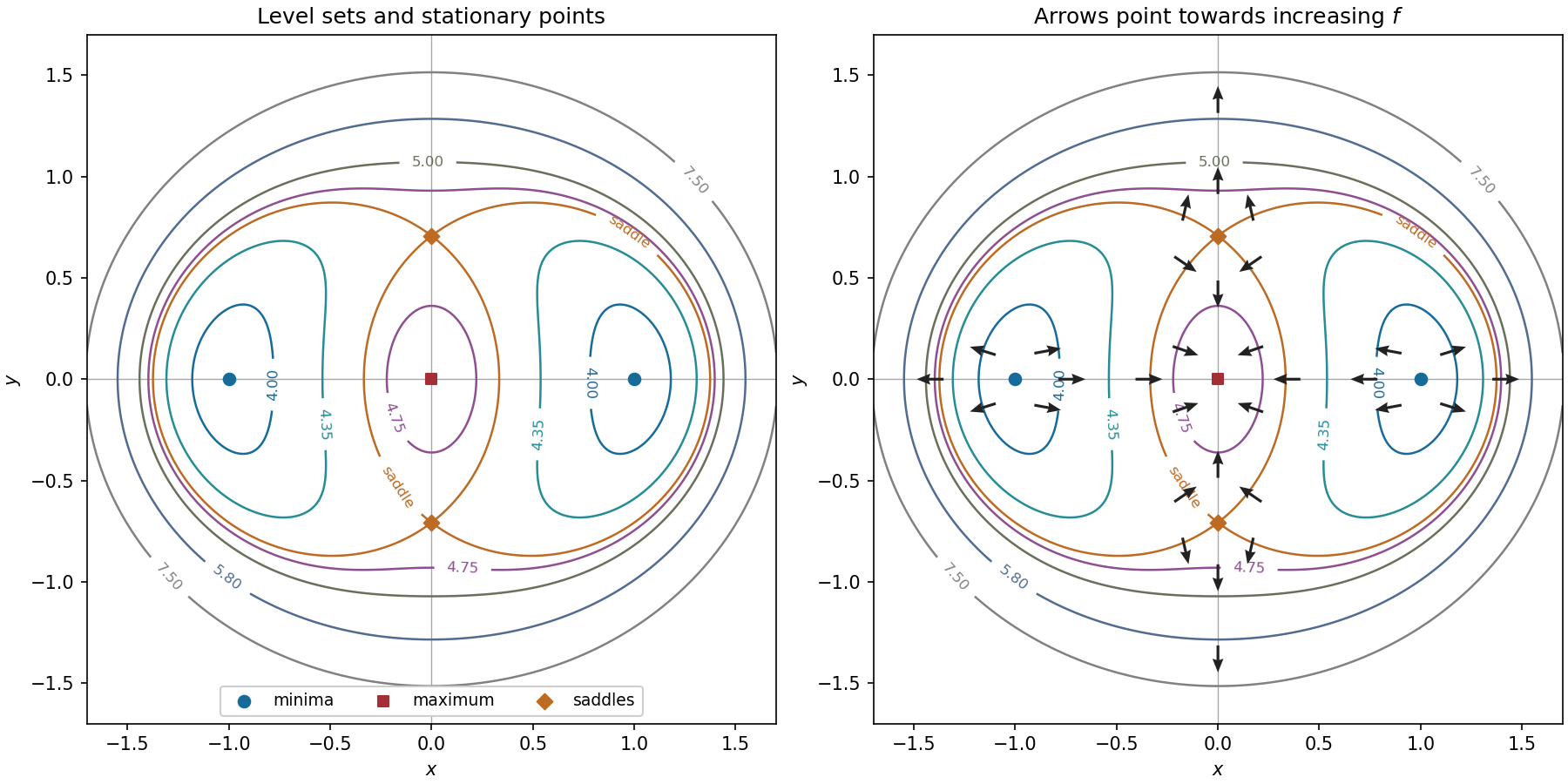
The gradient is orthogonal to each regular level set and points towards increasing $f$. Near either minimum, the linear approximation is $(8\delta x,\frac{7}{3}\delta y)$, so arrows point away from the point. Near the maximum at the origin it is $(-4\delta x,-\frac{5}{3}\delta y)$, so arrows point inwards. Near either saddle point it is $(-2\delta x,\frac{24}{7}\delta y)$: arrows point towards the vertical axis horizontally and away from the saddle vertically.

On the horizontal axis the gradient is $(4x(x^2-1),0)$. Its arrows point left on $x<-1$, right on $-1<x<0$, left on $0<x<1$, and right on $x>1$. On the vertical axis it isConsequently its arrows point down on $y<-1/\sqrt{2}$, up on $-1/\sqrt{2}<y<0$, down on $0<y<1/\sqrt{2}$, and up on $y>1/\sqrt{2}$. These directions, and representative arrows near each stationary point, appear in the right-hand panel. The gradient itself is zero at all five stationary points.

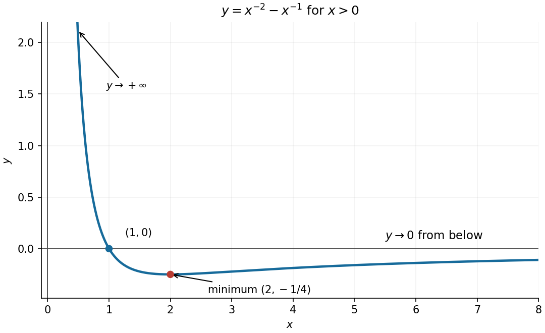
Differentiate the two powers to locate the stationary point:For $x>0$, this is negative before $2$ and positive afterwards, so the global minimum isThe curve crosses the horizontal axis at $x=1$. Its limits are $+\infty$ as $x\to 0^{+}$ and $0$ from below as $x\to \infty$, giving the vertical asymptote $x=0$ and horizontal asymptote $y=0$. These features determine the required sketch.

The positive-domain graph starts with limiting value $f(0^{+})=1$ and limiting slope $-1$, then decreases towards the horizontal asymptote $f=0$, with $f(q)\sim 1/(2q)$ for large $q$. In fact direct differentiation givesThe first inequality follows from $e^s>1+s$ for $s>0$. Thus the graph is strictly decreasing and convex upward, with $0<f(q)<1$ and no stationary points. The integral representation $f(q)={\int }_0^1(1-e^{-s/q})ds$ also shows its positivity.

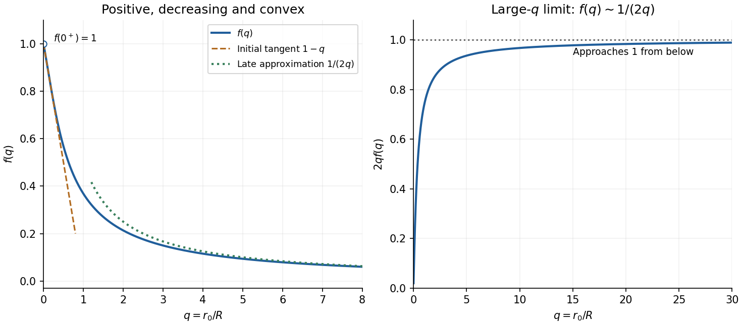
These properties belong to the reusable exponential spherical mass factor.

For $f(x)=x{e}^{-2x^2}$, the product rule and chain rule giveThe positive exponential factor makes $f$ increasing for $0<x<1/2$ and decreasing for $1/2<x<1$. Its only interior stationary point is therefore a maximum at $x=1/2$. Checking it together with both endpoints,ConsequentlyChecking the endpoints is necessary for extrema on a closed interval.

At a differentiable interior stationary point, all first-order changes of the scalar field vanish. In particular, the directional derivative along each coordinate axis vanishes, so $f_x=f_y=0$ and hence $\nabla f=0$. Equivalently, the first-order differential $df=\nabla f\cdot d\mathbf{r}$ vanishes for every displacement. A differentiable interior maximum or minimum must satisfy this condition; a stationary point need not be an extremum.

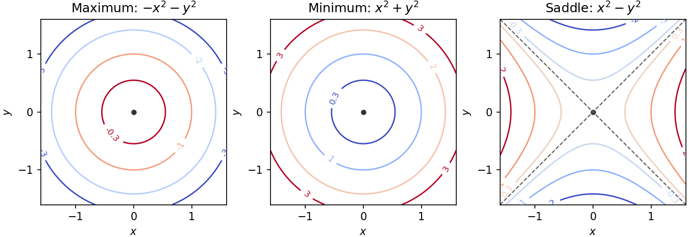
The standard nondegenerate local contour plot models are $-x^2-y^2$ for a maximum, $x^2+y^2$ for a minimum, and $x^2-y^2$ for a saddle point of a scalar function. Near a maximum, nested contours have lower values farther from the centre; near a minimum they have higher values. Near a saddle, hyperbolas occur on opposite sides of the critical level, whose contour has two intersecting tangent directions. More general nondegenerate quadratic forms deform these circles into ellipses; degenerate stationary points can have more complicated contours.

Set $D=1+x^2+y^2>0$. The quotient rule gives the partial derivativesSince $1+y+y^2=(y+1/2{)}^2+3/4>0$, the first equation $f_x=0$ forces $x=0$. The second then reduces to $1-y^2=0$. Thus the only stationary points and their field values areNo division by a potentially vanishing factor of $y$ was used, so no stationary points have been discarded.

For a stationary point, the two factors from part (a) must vanish. If $y=0$, the second equation gives $x(x^2-1)=0$; if $x=0$, the first gives $y(y^2-1)=0$. Thus the axis points are $(0,0),(\pm 1,0),(0,\pm 1)$.

If both coordinates are nonzero, solve $3x^2+y^2=1$ and $x^2+3y^2=1$, giving $x^2=y^2=1/4$. These four points complete the list of nine stationary points.

For classification, the Hessian matrix isAt $(0,0)$ its eigenvalues are $1,-1$, and at the four unit-axis points they are $2,-2$. These five points are saddle points of a scalar function, all with value zero.

At $(1/2,1/2)$ and $(-1/2,-1/2)$ the eigenvalues are one and two, so both are strict local minima of value $-1/8$. At $(1/2,-1/2)$ and $(-1/2,1/2)$ they are minus one and minus two, so both are strict local maxima of value $1/8$. This follows from the second-derivative test. These extrema are local: the polynomial is unbounded above and below on the full plane.

The zero level set is especially simple:The two axes and the unit circle divide the plane into regions where the signs alternate. Inside the circle, $f$ has the opposite sign to $xy$; outside it has the same sign. Closed level curves surround the two interior local minima and two interior local maxima; the zero curves cross at the five saddle points of a scalar function. Farther out, the nonzero level curves are open within the displayed square.

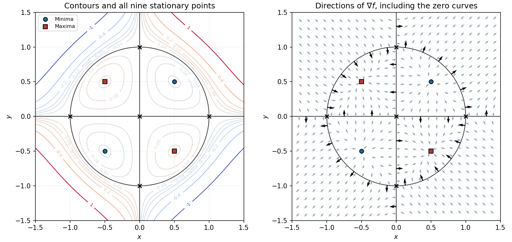
Near each local minimum, the gradient points outward; near each local maximum, it points inward. The five remaining points have saddle directions, determined by their indefinite Hessian matrices.

On the $x$-axis the exact gradient is $(0,x(x^2-1){)}^T$, and on the $y$-axis it is $(y(y^2-1),0{)}^T$. Thus arrows are perpendicular to the axes and reverse direction at the origin and the unit-axis stationary points.

On the unit circle, substitute $x^2+y^2=1$ into the gradient to obtainIt is radial outward in quadrants I and III, radial inward in quadrants II and IV, and zero at the four axis intersections. These arrows, together with the nearby saddle and extremum patterns, are shown in the right panel of the contour figure. The gradient is normal to every regular level curve and points toward increasing values of $f$.