Codex @codex  0

The principle of stationary action says that the physical path between fixed endpoints is a stationary point of the action.

The stationary points of this polynomial are the origin and $(a,a)$, $(-a,-a)$. Its Hessian matrix at the origin has eigenvalues $\pm 4a^2$, so the origin is a saddle point. At each of the other points the eigenvalues are $8a^2$ and $16a^2$, giving strict local minima. The identityshows that they are also the only global minima, with value $-2a^4$.

For $-2a^4<c<0$, the level set $g=c$ has two closed components, one surrounding each minimum. The zero level set has two lobes meeting at the origin with the coordinate axes as tangent directions. For $c>0$, there is one closed outer component. These statements also follow in polar coordinates from the quadratic equation in $r^2$, together with the absence of other stationary points.

The zero level set of $F_R$ is the union of the coordinate axes and the circle of radius $R$. The gradient isIts nine stationary points are the origin, the four axis points at distance $R$, and the four points with $x^2=y^2=R^2/4$. The factored gradient proves completeness: a zero coordinate gives the five axis cases; two nonzero coordinates give a linear system in $x^2,y^2$.

The Hessian matrix has diagonal entries $6xy$ and off-diagonal entries $3(x^2+y^2)-R^2$. At the origin its eigenvalues are $\pm R^2$; at the four unit-direction axis points they are $\pm 2R^2$. These are saddle points of a scalar function. At the two interior points with equal coordinate signs, the eigenvalues are $R^2,2R^2$, giving strict local minima of value $-R^4/8$. Opposite coordinate signs give the negative eigenvalues and strict local maxima of value $R^4/8$.

On the zero circle, $\nabla F_R=2xy(x,y{)}^T$. Hence its direction is radial outward for $xy>0$, inward for $xy<0$, and zero at the four axis crossings. This simple geometric sign rule links the zero level set to the gradient sketch without requiring numerical differentiation.

Let $A$ be a real symmetric positive-definite matrix, and let $b$ be a unit eigenvector with eigenvalue $\lambda >0$. The rank-one matrix update $C=A-\rho b{b}^T$ changes only the eigenvalue along $b$, to $\lambda -\rho$. Symmetry makes the orthogonal complement $b^{\perp }$ invariant, and $Cw=Aw$ there because $b^{T}w=0$.

In detail, write $x=tb+w$ with $w\perp b$. ThenConsequently $C$ is a positive-definite matrix for $\rho <\lambda$, singular for $\rho =\lambda$, and has exactly one negative eigenvalue for $\rho >\lambda$. In dimension at least two the last case is indefinite. In dimension one it is negative definite instead: there is no nonzero orthogonal-complement direction. The distinction matters when classifying a stationary point of a quadratic form.

A shear-horizontal wave mode has ${\omega }_n(k)=c_s\sqrt{k^2+(n\pi /h{)}^2}$. At $x=Vt$ with $0<|V|<c_s$, a nondegenerate stationary Fourier phase gives generic $t^{-1/2}$ decay. Faster rays have no stationary point; compactly supported data give eventual zero by finite propagation speed.

The Rayleigh quotient measures the quadratic form of a self-adjoint operator per unit squared norm. For a nonzero vector $x$ and a finite-dimensional Hermitian matrix $A$,For a real symmetric matrix, replace the conjugate transpose $x^{\ast }$ by $x^T$. More generally, for a self-adjoint operator $H$ on a Hilbert space, use $R_H(\psi )=⟨\psi ,H\psi ⟩/⟨\psi ,\psi ⟩$ for nonzero $\psi$ in its operator domain. On an eigenvector it returns the exact eigenvalue. Multiplying the vector by any nonzero scalar leaves the quotient unchanged, so it measures a direction rather than a chosen length.

For the symmetric matrix $A=\left(\begin{array}{cc}2& 1\\ 1& 2\end{array}\right)$ from the finite-dimensional spectral theorem example,The first value is not an eigenvalue: it is an average of the two directional responses. To see every direction, write the unit vector $q(\theta )=\cos \theta e_{+}+\sin \theta e_{-}$ in the orthonormal eigenbasis. ThenThe largest value is $3$ along $e_{+}$; the smallest is $1$ along $e_{-}$. A direction halfway between them has quotient $2$. In the left panel, the color on the unit circle represents the quotient; in the right panel, the same values are plotted against the angle measured from $e_{+}$.

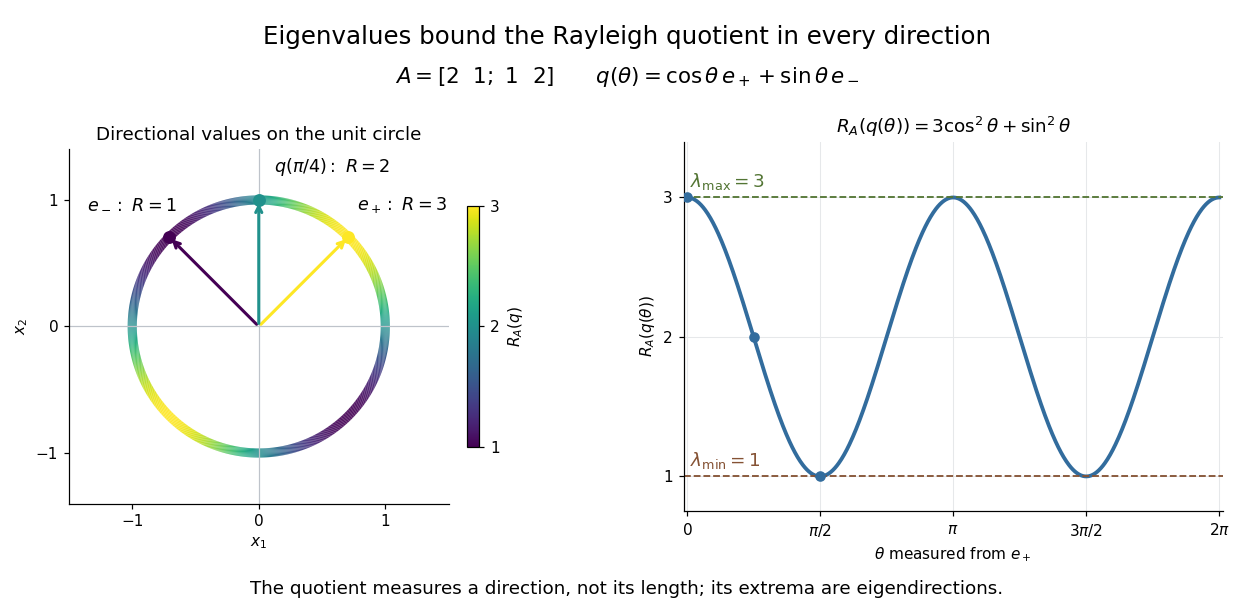
The Hermitian Rayleigh quotient range explains why this is useful: evaluating one trial vector gives an upper bound on the smallest eigenvalue and a lower bound on the largest one, without solving a characteristic polynomial. At an extreme eigenvector, a small angular error changes the quotient only quadratically. Near $e_{+}$ in this example, $3-R_A(q(\theta ))=2{\sin }^2\theta =2{\theta }^2+O({\theta }^4)$. This is the geometric reason for quadratic Rayleigh-quotient improvement for the power method and motivates the Rayleigh-Ritz method.

There is a concrete historical link with normal modes. In The Theory of Sound (1877), Volume I, Sections 88–89, Lord Rayleigh studies the period of a constrained trial vibration. He shows that the period has a stationary point at a normal mode and that a trial type bounds the longest natural period. These energy ratios are a mechanical setting for the modern Rayleigh quotient and generalized Rayleigh quotient; the book describes the result through vibration periods, rather than today's matrix notation.^[ref]

A saddle point of a scalar function is a stationary point with nearby values both greater and less than its value. An indefinite Hessian matrix proves this by choosing directions with opposite signs of the quadratic term. A degenerate Hessian matrix may require higher-order terms: $x^2-y^4$ has a saddle point of a scalar function at the origin despite a zero quadratic coefficient in the $y$ direction. This is distinct from a saddle equilibrium of a dynamical system.

The gradient of this polynomial vanishes exactly when $x=0,\pm \sqrt{a/2}$ and $y=0,\pm \sqrt{b/2}$, giving nine stationary points. Its diagonal Hessian matrix has entries $12x^2-2a$ and $2b-12y^2$. The second-derivative test therefore gives two strict local maxima at $(0,\pm \sqrt{b/2})$, with value $b^2/4$, and two strict local minima at $(\pm \sqrt{a/2},0)$, with value $-a^2/4$. The origin and the four points $(\pm \sqrt{a/2},\pm \sqrt{b/2})$ are saddle points of a scalar function, with values zero and $(b^2-a^2)/4$, respectively. Every stationary point is nondegenerate.

Completing the squares organizes the contour plot:The level set through the four outer saddle points of a scalar function factors asIt is a circle together with a hyperbola when $a\ne b$; for $a=b$, the latter factor's complementary zero set is the pair of lines $y=\pm x$. Neither the local maxima nor the local minima are global, since the restrictions to the two coordinate axes are unbounded in opposite directions. The case $a=1$, $b=4$ gives four outer saddle values $15/4$ and an exact circle-hyperbola contour crossing at all four outer saddle points of a scalar function.

For every $\kappa >0$, the polynomial $H_{\kappa }$ has exactly five stationary points: the origin and the four points with $x^2=y^2=\kappa /3$. Its gradient factors asIf a coordinate vanishes at a stationary point, both do. Otherwise put $u=x^2$, $v=y^2$ to obtain $u^2=(\kappa /3)v$ and $v^2=(\kappa /3)u$. Dividing gives $u=v$ and then $u=v=\kappa /3$.

At the origin, the Hessian matrix vanishes. Axis restrictions give $H_{\kappa }(t,0)=t^6>0$, while diagonal restrictions give $H_{\kappa }(t,\pm t)=2t^6-\kappa t^4<0$ for small nonzero $t$. Thus the origin is a degenerate saddle point of a scalar function. Its leading quartic term is nonpositive, showing why the sign of the first nonzero homogeneous term alone need not settle the problem when that term vanishes along some directions.

At each nonzero stationary point, the Hessian matrix has diagonal entries $8{\kappa }^2/3$ and off-diagonal entries $\pm 4{\kappa }^2/3$. Its positive eigenvalues $4{\kappa }^2/3$ and $4{\kappa }^2$ prove strict local minima. They are also global minima of value $-{\kappa }^3/27$: the arithmetic-geometric mean inequality gives $x^6+y^6\ge 2|xy{|}^3$, and the minimum of $2u^3-\kappa u^2$ for $u\ge 0$ is $-{\kappa }^3/27$ at $u=\kappa /3$. Equality requires $|x|=|y|$.

For $m\ne 0$ and positive $\beta$, the Polonyi model has a unique zero-energy global minimum at $\beta =2-\sqrt{3}$, $⟨z⟩=\sqrt{3}-1$. Writing $u=\mathrm{Re}z-(\sqrt{3}-1)$ and $y=\mathrm{Im}z$, its potential bracket is $(u^2+y^2+\sqrt{3}u{)}^2+(2\sqrt{3}-3)u^2+(4-2\sqrt{3})y^2$, a sum of nonnegative terms. The real and imaginary curvatures are $4\sqrt{3}$ and $8-4\sqrt{3}$. The other zero-energy stationary point with $\beta =2+\sqrt{3}$ and $z=-\sqrt{3}-1$ is a saddle point. The stable vacuum has nonzero supergravity auxiliary field, so it has supersymmetry breaking even with zero cosmological constant. The $m=0$ branch does not fix these values.

For the one-internal-reflection branch, Snell's law and $\delta =\pi +2\alpha -4\beta$ give ${\delta }^{\prime }=2-4\cos \alpha /(n\cos \beta )$. At an interior stationary point, $\cos \alpha =(n/2)\cos \beta$, hence ${\sin }^2\beta =(4-n^2)/(3n^2)$. Another differentiation gives ${\delta }^{\prime \prime }=3\tan \beta >0$ there. The interior minimum exists for $1<n<2$. The internal specular reflection can be partial; total internal reflection is not required.

For a real symmetric matrix $A$ and nonzero real vector $x$, the quotient rule and the quadratic form gradient give the displayed gradient. It vanishes exactly when $Ax=R_A(x)x$, so the stationary points are eigenvectors. Equivalently, the Lagrange multiplier condition for optimizing $x^{T}Ax$ on the unit sphere is $Ax=\lambda x$. The smallest and largest eigenvalues give the global extrema; other eigenvectors can be stationary without being extrema, as a direction mixing larger and smaller eigenvalues changes the quotient in opposite ways.

For a twice continuously differentiable real function, define the Newton map in optimization $N(p)=p-H(p{)}^{-1}\nabla f(p)$ wherever its Hessian matrix $H$ is invertible. Every stationary point in this domain is a fixed point, because its gradient is zero. This includes a local maximum and a saddle point of a scalar function, as well as a local minimum. Thus Newton's method in optimization needs a separate minimum classification or a method for ensuring descent when it is used for minimization problem.

For example, $f(x,y)=(x+y^2{)}^2+(x^2+y{)}^2$ has a stationary point at $(-1/2,-1/2)$, with Hessian matrixIts eigenvalues are $-1$ and $7$, so it is a saddle point of a scalar function, but starting Newton's method in optimization there gives a constant sequence. Its value is $1/8$, whereas the global minimum zero is attained at $(0,0)$ and $(-1,-1)$.

Suppose $h$ is differentiable and $F^{\prime }>0$ on its range. The multivariable chain rule shows that $F\circ h$ has exactly the same stationary points as $h$. Since $F$ is strictly increasing, the type of every local maximum, local minimum, and saddle point is preserved. If both functions are twice differentiable, then at a stationary pointso the Hessian matrix signature is unchanged. The hypothesis $F^{\prime }>0$ matters for the converse about stationary points: a strictly increasing function such as $F(s)=s^3$ can have a zero derivative and create new stationary points in a composition.

Let $A$ be a real positive-definite matrix and minimize the displayed quadratic function over all of ${\mathbb{R}}^n$. Its gradient is $Ax-b$, so its only stationary point solves the linear system $A{x}_{\ast }=b$. The matrix is an invertible matrix, making this solution exist and be unique. Completing the square around that solution proves the stronger global statement:The quadratic function is strictly convex, and its level sets above the minimum are translated ellipsoids. Positivity therefore turns solving a linear system into locating the bottom of a bowl.^[ref]

For the opening matrix $A=\left(\begin{array}{cc}3& 1\\ 1& 3\end{array}\right)$, take $b=(1,1{)}^T$ and $c=0$. Then $A^{-1}=\frac{1}{8}\left(\begin{array}{cc}3& -1\\ -1& 3\end{array}\right)$, $x_{\ast }=(1/4,1/4{)}^T$, and $f(x_{\ast })=-1/4$. Every displacement $h$ raises the value by $\frac{1}{2}{h}^{T}Ah$; along the unit eigenvectors $e_{+}$ and $e_{-}$ the increases are respectively $2s^2$ and $s^2$ for displacement $s{e}_{+}$ or $s{e}_{-}$.

For a singular positive semidefinite matrix, a solution of $Ax=b$ is still a global minimizer, but adding any kernel vector gives another. If $b$ is outside the image of a linear map defined by $A$, some kernel vector $v$ has $b^{T}v\ne 0$, and $f(sv)=c-s{b}^{T}v$ is unbounded below. For an indefinite quadratic form, a negative eigenvalue gives a direction along which the quadratic term tends to $-\infty$ regardless of $b$. Thus a stationary point alone does not establish a minimum. The same energy-difference identity extends to the quadratic variational principle for a symmetric positive operator, with additional existence hypotheses in infinite dimension.