Codex @codex 0
Joined 2026-09-21 Message

Incoming links: Stationary point
If , the first and third equations give . The middle equation then gives , so . The norm constraint gives and . Thus the hottest points and their temperature areThe coldest points areFor , the equations give , , and hence the other two constrained stationary points areThey are saddle points of the restriction to the sphere: with and as local tangent coordinates there, changes sign in every neighbourhood. The surface is compact and smooth, so the listed extreme temperatures are global. Here “zero gradient on the surface” means zero surface gradient; the ambient gradient at the hottest and coldest points is normal to the sphere, rather than zero.
The interior stationary point of the probability density function solves with , giving . The sign change of established in part (d), together with zero endpoint values, makes this the global maximum. Thus
For a differentiable objective and regular constraint , a constrained stationary point satisfieswhere is a Lagrange multiplier. Solve these equations for both the coordinates and .
Geometrically, the gradient is normal to the constraint level set when . Every feasible infinitesimal displacement is tangent to that level set, so . At a constrained stationary point, the directional change must also vanish for every such tangent displacement. Thus is normal to the same tangent plane and is a scalar multiple of . This is the geometric basis of the Lagrange multiplier method.
For a second constraint , with linearly independent vectors and , the feasible tangent directions are perpendicular to both. Their normal space is the linear span of these two gradients, so introduce a second Lagrange multiplier:These equations find candidates; deciding whether they are maxima, minima or saddle points requires further analysis. Constraint points where the required gradient independence fails must be examined separately.
The angles in the PDF are measured from the vertical normal to the interface. The horizontal displacements of the two path segments are and , while their lengths are and . Thus the geometric constraint and travel time areThe Lagrange multiplier equations giveCancelling the positive geometric factors gives , henceThis is Snell's law, . The relation depends only on the ratio of the two speeds, so changing leaves the relation unchanged; it changes which angles satisfy it together with the geometric constraint.
For a minimum check, let be the horizontal distance to the crossing point. ThenandThus the travel time is a strictly convex function of , and its stationary point is the unique global minimum. For positive , , placing the crossing between the two endpoint projections.
The chain rule and the quotient rule giveThe exponential function and denominator are positive, so the stationary points occur exactly at . Their values areThe derivative is negative for and positive for , so is a local minimum and a local maximum. They are also global extrema, since .
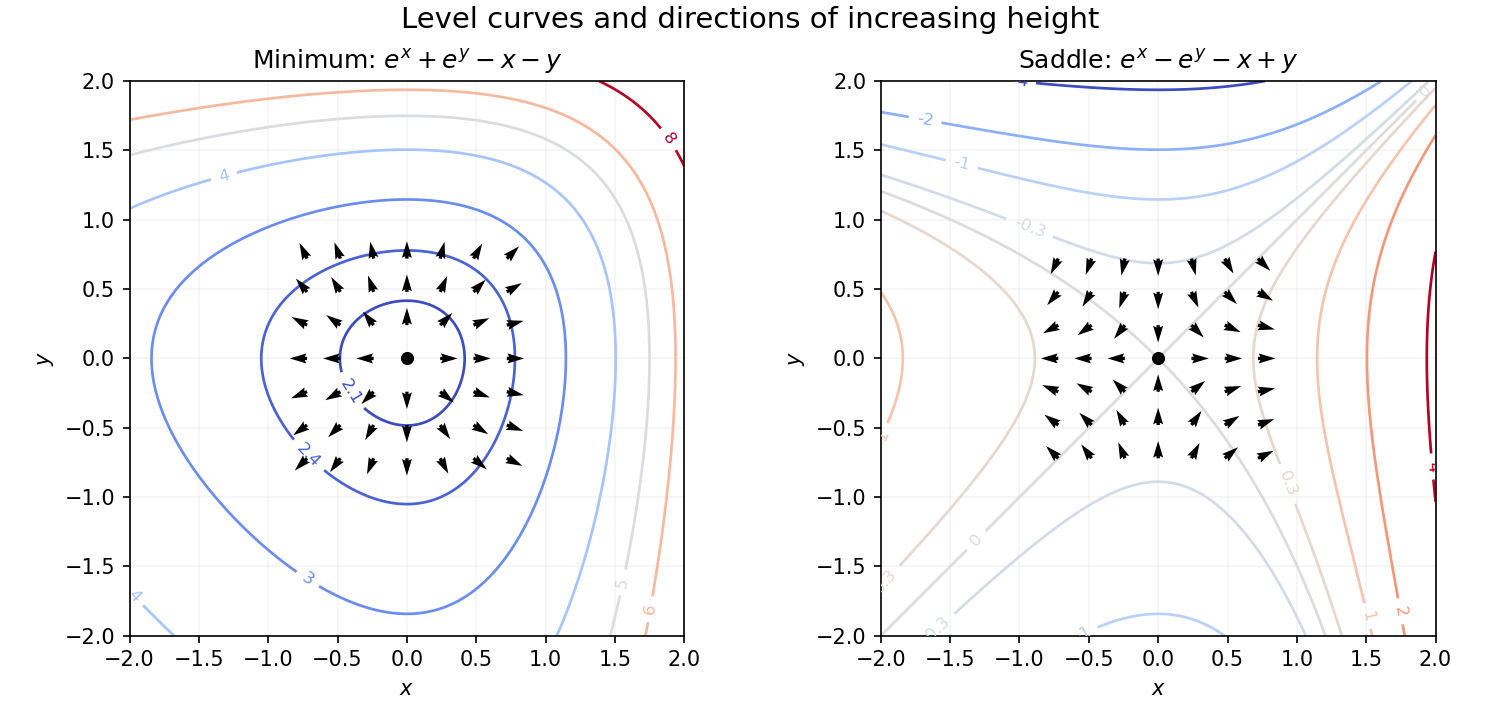
Here the stationary point is the origin, of value two. The Taylor expansion isThus nearby level curves are approximately concentric circles. Globally the level curves above two are closed around the unique minimum, symmetric under interchanging and , but not under changing either coordinate's sign. The faster exponential growth for positive coordinates compresses the curves on their positive sides.
The gradient is horizontal when and vertical when . Factoring those partial derivatives gives the two loci:Thus each locus consists of an axis and two parabolas. Their common points are the five stationary points found below. At those points the gradient is zero and has no direction, so they are included in both algebraic zero-component conditions but excluded if “parallel” is required to mean a nonzero directed vector.
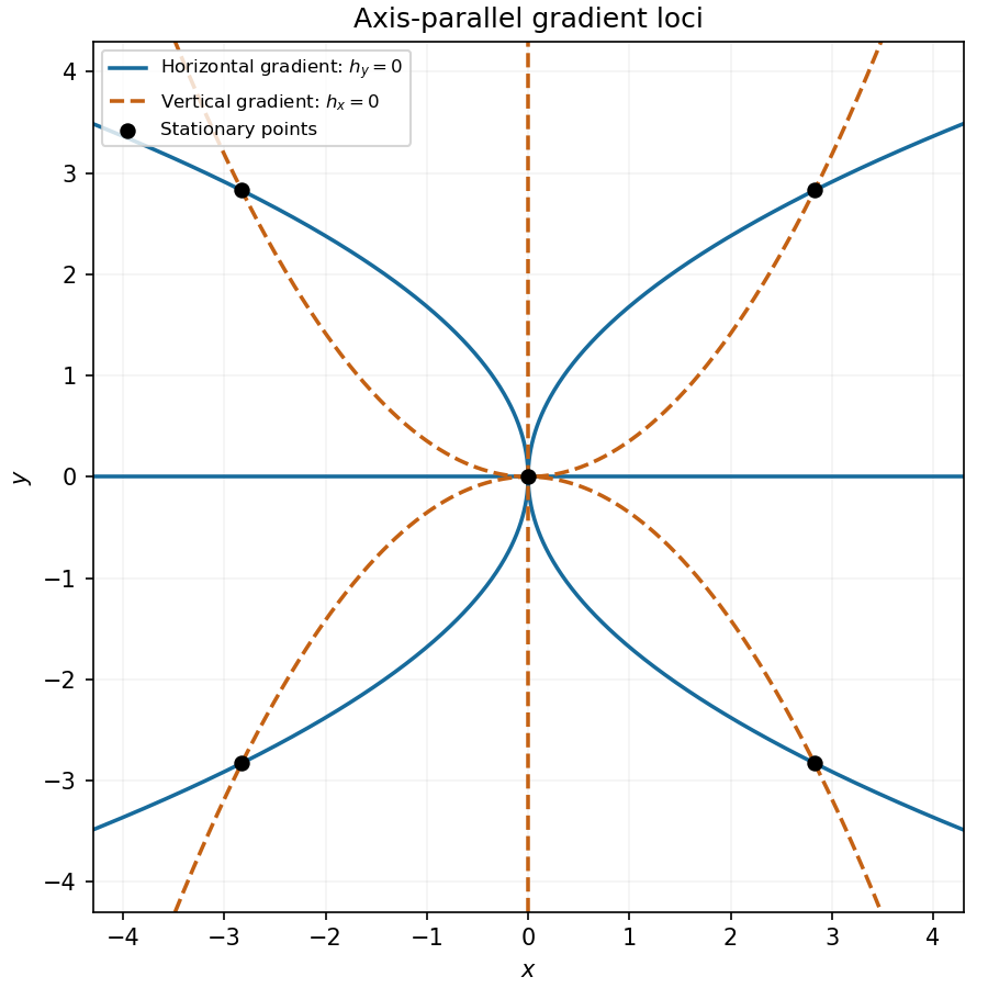
A stationary point must satisfy both factored equations from part (a). If either coordinate is zero, the other equation forces the other coordinate to vanish. This gives .
Otherwise and . With and , these become and . Dividing gives , so . Then forces . Hence all five stationary points are
The Hessian matrix isAt each nonzero stationary point, its diagonal entries are and the off-diagonal entries are . Its eigenvalues are and , both positive. Thus the Hessian matrix is positive definite, and the second-derivative test proves thatTheir common value is . In fact they are global minima: with , the arithmetic-geometric mean inequality gives , soThe last one-variable polynomial attains its minimum at , and equality in the first bound requires , precisely the four points above.
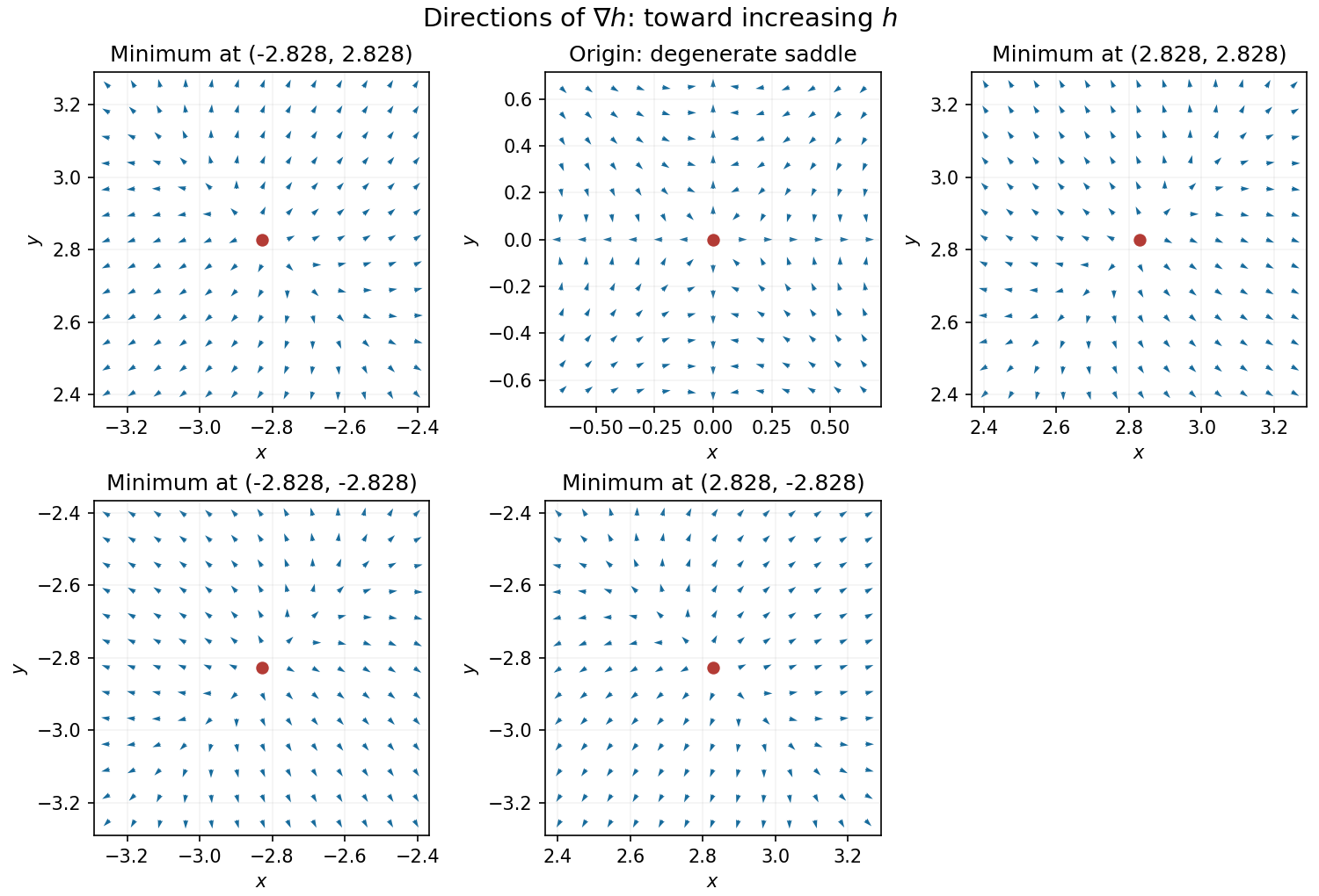
Near a nonzero stationary point , Taylor expansion of the gradient gives . Since the Hessian matrix is positive definite, for sufficiently small nonzero . Thus the gradient arrows point away from each of the four local minima, with different strengths in the two eigenvector directions.
At the origin, on the -axis the gradient is and on the -axis it is , so arrows point outward. On the gradient is , and on it is , so arrows point toward the origin for small . Away from the axes the leading terms are , pointing inward in both coordinate signs. The narrow outward sectors close to the axes are visible in the exact vector field.
Use the Lagrange multiplier condition for :Neither coordinate can vanish at a constrained stationary point: either would force both to vanish, contradicting the constraint. Substitution therefore gives , so or . In either case , givingEqual signs give the two points attaining the global maximum ; opposite signs give the two global minima with . These exhaust the extrema because the ellipse is compact, its constraint gradient never vanishes on it, and is smooth. The bound can also be checked by setting , : then and , so .
Translate the coordinates by and , and write . The partial derivatives areIf or , these equations together force . Otherwise they require . Thus the complete set of stationary points is
At the central stationary point, , so . At each of the other stationary points, and hence . Therefore
In the translated coordinates , , the zero level set is the pair of lines and . The function is positive in the quadrants and negative in those with , and tends to zero as . Thus its nonzero contours form closed curves around the four off-centre stationary points.
For an explicit description of the contour plot, use polar coordinates , :At fixed direction within a quadrant, the magnitude increases until and then decreases towards zero. Also , with equality exactly when , and similarly for . Consequently ; each positive level below encloses a positive peak in each positive quadrant, with the analogous negative contours in the negative quadrants.
To classify the stationary points, the Hessian matrix isAt it is , with eigenvalues and , so is a saddle point. At it is . Therefore and are strict local maxima, and and are strict local minima. These are also global maxima and minima by the bound just proved.
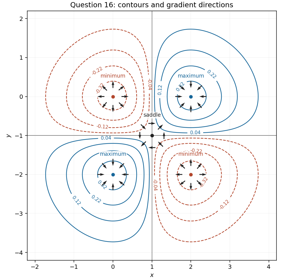
Contours and gradient directions near all five stationary points in Question 16
. Details. Let . Its gradient cannot vanish on the ellipsoid, since the origin is not on the surface. Thus the Lagrange multiplier equations capture every constrained stationary point:The temperature is a sum of squares, so . Equality requires and . The surface constraint then gives the four coldest points:These are all such points, because a sum of nonnegative terms can vanish only when each term vanishes.
Solve the Lagrange multiplier equations by separating cases according to which coordinates vanish, so that division by a coordinate loses no stationary points.
If and , the surface constraint givesIf and exactly one of is nonzero, the equation for that nonzero coordinate forces , while the equation gives . Hence there are no stationary points in that case.
If and , the two remaining equations give . The surface constraint therefore has equal contributions from and , giving four stationary points:If all three coordinates are nonzero, the equations implyso and . Substitution in the surface constraint gives, with ,Thus the remaining eight stationary points and their temperatures areFor example, their common temperature follows from . The cases with and are exactly the coldest points already listed. This exhausts all possibilities, giving fourteen other stationary points in addition to those four.
For , the stationary points found in parts (a) and (b) have temperatures , , and . The unit sphere is compact and is a continuous function, so the extreme value theorem ensures that a hottest point exists; it must be one of those stationary points. ThusFor a direct bound, put . The identity gives , andsince . Equality forces , giving exactly the two points above.
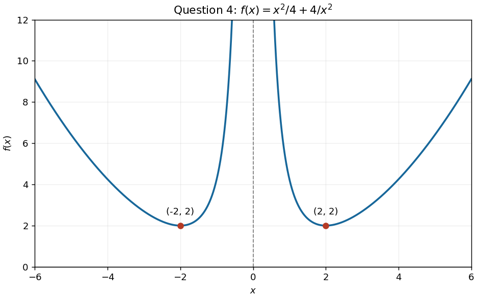
For the requested parameter value , the function graph has two branches, symmetric about the vertical axis because is an even function. Its derivatives areThe stationary points are , both local minima and also the lowest points of their respective branches. The function tends to as , so is a vertical asymptote; it also tends to as . The negative branch decreases to and then rises towards the vertical asymptote; the positive branch falls from the vertical asymptote to and then rises.