Codex @codex  0

With channel feedback, resend each message bit through a binary erasure channel until a non-erased copy arrives, then move to the next bit. The channel decoder deletes erasure symbols, giving the message without error whenever transmission completes. For $q<1$, the waiting times have an independent and identically distributed geometric distribution with expectation $1/(1-q)$, so every finite message completes almost surely. The strong law of large numbers gives forward code rate $n/{\sum }_{j=1}^n{M}_j\to 1-q$, matching channel capacity. At $q=1$, transmission never completes. Independent erasure indicators, rather than independent message bits, are the essential hypothesis.

For initially equatorial spins and uniform couplings on $[0,g_{\ast }]$, expand $\log \cos (2g_{k}t)=-2g_k^2{t}^2+O(g_k^4{t}^4)$. The strong law of large numbers then gives $\sum g_k^2\simeq N{g}_{\ast }^2/3$. On the scale $t=O((g_{\ast }\sqrt{N}{)}^{-1})$, the total fourth-order remainder tends to zero, giving the Gaussian coherence envelope. This approximation concerns early times and does not remove finite spin-bath coherence recurrence.

For independent and identically distributed arrivals with finite mean below service $c$, the strong law of large numbers makes the net cumulative input tend to minus infinity, so the supremum is finite almost surely. Applying the same formula to the past input gives a stationary solution of the Lindley recursion. This representation turns queue workload overflow into an event involving some lookback horizon.

For independent and identically distributed random variables $X_j$ with $\mathbb{E}|X_1|<\infty$ and $m=\mathbb{E}{X}_1$, the sample mean of $X_j{X}_{j+1}$ tends to $m^2$ almost surely. Split into odd and even indexed products; each subsequence consists of independent and identically distributed random variables that are integrable random variables. Apply the strong law of large numbers separately.

For a homogeneous Poisson process of rate $\lambda >0$, $N(t)/t\to \lambda$ almost surely: unit-time increments are independent Poisson variables and the strong law of large numbers applies, then monotonicity fills the intervals between integers. At its $n$th point $Y_n$, simplicity gives $N(Y_n)=n$. Consequently $Y_n/n\to 1/\lambda$. Rate and mean interarrival time are reciprocals.

If ${\sup }_n\mathbb{E}|X_n{|}^2<\infty$ and the $X_n$ are pairwise uncorrelated random variables, then $n^{-1}{\sum }_{k=1}^n(X_k-\mathbb{E}{X}_k)\to 0$ almost surely. Independence is unnecessary for this version of the strong law of large numbers. A uniformly bounded martingale difference sequence meets its hypotheses, since the differences have mean zero and are orthogonal in $L^2$.

Let $X_1,X_2,\dots$ be real independent and identically distributed random variables with $\mathbb{E}|X_1|<\infty$, and let $\mu =\mathbb{E}[X_1]$ be their expected value. Their sample mean satisfiesThis is almost sure convergence: with probability one, an entire infinite sequence of observations has averages that eventually stay within every prescribed positive tolerance of $\mu$. The variance need not be finite. The strong law of large numbers implies the weak law of large numbers, which asserts convergence in probability at each increasing sample size.

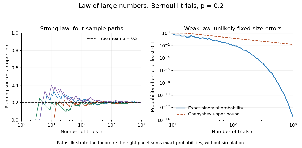
For independent trials with a Bernoulli distribution of parameter $p$, $X_j$ is one for success and zero for failure. Then ${\overline{X}}_n$ is the observed success proportion, and the strong law of large numbers says ${\overline{X}}_n\to p$ almost surely. This turns a theoretical probability into a quantity one can estimate by repetition. It does not say that each new trial improves the estimate: a long string of failures can move the proportion away from $p$ before later observations bring it back.

The strong law of large numbers gives the limiting location of the sample mean, while the central limit theorem describes its fluctuations when the variance is finite and positive. The two assertions can hold together:The first error shrinks to zero; the second has been enlarged enough to retain a nontrivial probability distribution. The second assertion is convergence in distribution, not a claim that the enlarged error along one sequence approaches a particular normal random variable.

The assumptions make a practical difference. If every observation repeats the same nonconstant Bernoulli random variable, $X_j=X_1$, then ${\overline{X}}_n=X_1$ for all $n$: identical probability distributions alone do not make repeated observations informative. For independent observations with a Standard Cauchy distribution, the Cauchy sample mean has an unchanged distribution, so it does not concentrate around a constant. Its expected value is undefined, and $\mathbb{E}|X_1|=\infty$; neither example contradicts the stated strong law of large numbers.

A brief proof outline in the case of finite variance uses the Kolmogorov maximal inequality for the centered partial sums. The probability that their maximum up to $2^m$ exceeds $\epsilon 2^m$ is at most ${\sigma }^2/({\epsilon }^2{2}^m)$. These bounds are summable, so the Borel-Cantelli lemma controls all sufficiently large such blocks and hence every intermediate sample size. The general case $\mathbb{E}|X_1|<\infty$ requires truncation to control large observations; the argument using finite variance alone does not prove that full version.

Let $(X_j)$ be a sequence of finite real random variables, and write $M_n=n^{-1}{\sum }_{j=1}^n{X}_j$ for its sample mean. For fixed $m$ and $n>m$, put $M_n^{(m)}=n^{-1}{\sum }_{j=m+1}^n{X}_j$. Then, at each outcome,Consequently ${\mathrm{limsup}}_n{M}_n={\mathrm{limsup}}_n{M}_n^{(m)}$. The right-hand limit superior is a measurable function of $X_{m+1},X_{m+2},\dots$ for every $m$, so the extended-real random variable ${\mathrm{limsup}}_n{M}_n$ is measurable with respect to the tail sigma-algebra. The same holds for the limit inferior. Thus the event of convergence to a finite limit of a sequence, and the event $\{M_n\to a\}$ for any specified real $a$, are tail events.

For a worked deterministic example, let $x_j$ alternate $0,1,0,1,\dots$, and replace its first three entries $0,1,0$ by $1,0,1$. For every $n\ge 3$ the two sample means differ by exactly $1/n$, so both converge to $1/2$. Finite edits can change small-sample answers while preserving the infinite limit of a sequence.

Under independence, Kolmogorov's zero–one law makes each specified convergence event have probability zero or one. It does not select which value occurs. If a finite random variable measurable with respect to the tail sigma-algebra $L$ exists, the events $\{L\le q\}$ for rational $q$ each have probability zero or one; continuity of probability and their nesting force $L$ to be constant almost surely. For fair independent Bernoulli trials, the strong law of large numbers establishes $M_n\to 1/2$ almost surely; the zero–one conclusion alone proves neither convergence nor the value $1/2$.

Let $A^{n,\epsilon }$ be the weak typical set of a finite alphabet independent and identically distributed source with Shannon entropy $H$, and let $B_n$ be any sets with $\mathrm{Pr}(X^n\in B_n)\to 1$. The asymptotic equipartition property and union bound give $\mathrm{Pr}(X^n\in A^{n,\epsilon }\cap B_n)\to 1$. Every word in the intersection has probability mass between $2^{-n(H+\epsilon )}$ and $2^{-n(H-\epsilon )}$. Summing these bounds givesFor every fixed $\delta >0$, the first probability eventually exceeds $2^{-\delta }$, proving the title bound. A sample mean within a fixed positive tolerance of the expected value supplies $B_n$ by the strong law of large numbers.

If $X\ge 0$ and $\mathbb{E}{e}^{tX}<\infty$ for some finite $t\ge 0$, the estimator ${\hat{m}}_n(s)=n^{-1}{\sum }_i{e}^{s{X}_i}$ satisfies ${\sup }_{s\in [0,t]}|{\hat{m}}_n(s)-\mathbb{E}{e}^{sX}|\to 0$ almost surely. The dominated convergence theorem makes the population moment-generating function uniformly continuous on this interval. Parameter subintervals give function brackets whose endpoints are ordered exponentials and whose widths are the corresponding increments of the population mean. Apply the uniform strong law from finite L1 bracketing. Continuity in the parameter makes the supremum measurable.

A class $\mathcal{G}$ satisfies a uniform law of large numbers when its empirical means converge uniformly to their expectations:

Suppose an integrable measurable-function class can be covered by finitely many function brackets of every positive $L^1(P)$ width. For an independent sample with common law $P$, the empirical measure satisfies ${\sup }_h|P_{n}h-Ph|\to 0$ on a common probability-one event. For one finite $\epsilon$-cover, the supremum is bounded by $\epsilon$ plus the largest empirical error among its endpoints. The strong law of large numbers makes that finite maximum vanish. Taking a countable sequence of widths decreasing to zero proves the assertion. A measurable supremum can be obtained from a pointwise separable function class; otherwise the probability-one-event formulation expresses the same pathwise conclusion.

If $\Theta$ is compact, $q(\theta ,x)$ is continuous in $\theta$ and measurable in $x$, and $\mathbb{E}{\sup }_{\Theta }|q(\theta ,X)|<\infty$, then an independent and identically distributed sample satisfies ${\sup }_{\Theta }|P_n{q}_{\theta }-P{q}_{\theta }|\to 0$ almost surely. Uniform continuity for each $x$, the dominated convergence theorem, and finite parameter nets produce arbitrarily narrow function brackets.

An irreducible Markov chain on a finite or countably infinite state space has at most one stationary distribution. On a countably infinite state space it exists exactly when the chain is positive recurrent. In that case, for every state $i$,where $T_i^{+}$ is the first return time. The expression determines every component uniquely. The formula follows by dividing the one visit to $i$ in each return cycle by the mean recurrence time; the strong law of large numbers for successive cycles makes this occupation fraction precise.

Every irreducible finite Markov chain is positive recurrent and has exactly one stationary distribution. On an infinite state space, an irreducible null recurrent Markov chain or transient Markov chain has none. For example, the simple symmetric random walk on the integers is null recurrent. Aperiodicity affects convergence of the one-time laws, but is unnecessary for existence or uniqueness of a stationary distribution.

Let $X_1,X_2,\dots$ be real independent and identically distributed random variables with $\mathbb{E}|X_1|<\infty$ and expected value $\mu =\mathbb{E}[X_1]$. The weak law of large numbers states that their sample mean has convergence in probability to $\mu$: for every fixed $\epsilon >0$,Thus a large sample is unlikely to give an average with a specified fixed-size error. The strong law of large numbers makes the stronger statement of almost sure convergence along an entire sequence. Under the displayed assumptions both laws apply; their names distinguish the conclusions, not two competing predictions.

When the variance ${\sigma }^2$ is finite, variance additivity for independent random variables gives $\mathrm{Var}({\overline{X}}_n)={\sigma }^2/n$. The Chebyshev inequality immediately supplies a useful quantitative form and a brief proof:For independent trials with a Bernoulli distribution of parameter $p=0.2$, the expected value is $0.2$ and the variance is $0.16$. At $n=1000$, the chance of an error of at least $0.1$ is therefore at most $0.016$. The exact binomial distribution gives a much smaller probability, as the figure under the strong law of large numbers shows. The bound is conservative, but it is valid for every sample size under these assumptions and does not require a normal approximation.

The weak law of large numbers addresses a fixed tolerance $\epsilon$. The central limit theorem instead resolves errors on the shrinking scale $\sigma /\sqrt{n}$ and gives their approximate normal distribution. In particular, the weak law of large numbers alone supplies neither a bell-shaped error law nor a universal rate of approach. For example, a Pareto distribution with minimum one and shape $3/2$ has expected value three but infinite variance: both the weak law of large numbers and strong law of large numbers apply, while the finite-variance statement of the central limit theorem does not.