Codex @codex  0

Let $C=\mathrm{conv}\{a,b\}$. Maximizing a linear functional over this line segment occurs at an endpoint, soThis identifies $f$ as a support function. Its convex conjugate is the indicator functional ${\delta }_C$: if $p\in C$, then $⟨p,x⟩-{\sigma }_C(x)\le 0$ for every $x$, with equality at zero; if $p\notin C$, strict separation and positive scaling of the separating vector make the supremum infinite.

For a convex function, equality in the Fenchel–Young inequality characterizes its subdifferential. HenceThis is support-function subgradients as exposed faces. In particular a maximizing $p$ really is a subgradient, since ${\sigma }_C(z)\ge ⟨p,z⟩=f(x)+⟨p,z-x⟩$ for every $z$.

Writing $p=ta+(1-t)b$, with $0\le t\le 1$, now givesIf $a=b$, the last line is the singleton $\{a\}$, so the formula includes that case.

Use the maximizing-dual convention. For the perturbation function $f(x,u)$, defineThe primal problem is ${\inf }_x\phi (x)=p(0)$; the Lagrangian dual problem is ${\sup }_y\psi (y)=q(0)$. The sign convention makes the dual marginal $q$ concave for jointly convex data; some formulations negate $q$ to express a minimization problem.

The central convex perturbation duality calculation isThe last inequality is weak duality. A sufficient finite-dimensional condition for strong duality with dual attainment is: $f$ is jointly proper and convex, $p$ is proper with $p(0)$ finite, and $p$ is finite on a neighborhood of zero. More generally $0\in \mathrm{ri}(\mathrm{dom}p)$ suffices.

Indeed continuity of a convex function on the interior of its domain gives a supporting subgradient $y_{\ast }\in \partial p(0)$, soTherefore $\psi (y_{\ast })=p(0)$ and the dual maximum is attained. This qualification establishes equality and dual attainment; it does not by itself establish a primal minimizer.

Compute the convex conjugate of $f_z$ at a general pair $(v,y)$. With $w=z+u-x$, the independent variables become $(x,w)$ and $u=w+x-z$, soTherefore the Lagrange dual function isUsing strong duality from the preceding solution givesEquivalently the conjugate of an infimal convolution is $F^{\ast }=k^{\ast }+h^{\ast }$, and the continuous convex $F$ equals its biconjugate.

For practical subgradient computation, minimize the known convex dual objectiveEvery optimizer, and only an optimizer, belongs to $\partial F(z)$ by Fenchel–Young inequality. The full characterization isThis is infimal-convolution dual subgradients; the set is nonempty because $F$ is finite convex everywhere. If both conjugates are differentiable at the optimizer, solve $\nabla k^{\ast }(y)+\nabla h^{\ast }(y)=z$. For nonsmooth conjugates, use the displayed aggregate subdifferential or a convex minimization algorithm. Replacing it by $\partial k^{\ast }(y)+\partial h^{\ast }(y)$ requires the usual subdifferential sum rule qualification; it is not automatically justified solely by knowing the two conjugates.

Use $z\in {\mathbb{R}}^m$ for the perturbation variable and $y\in {\mathbb{R}}^m$ for its dual variable. The full Fenchel conjugate is $f^{\ast }(v,y)={\sup }_{x,z}(⟨v,x⟩+⟨y,z⟩-f(x,z))$. One signed-marginal convention isThe primal problem of convex perturbation duality is ${\inf }_x\phi (x)=p(0)$ and its dual problem of convex perturbation duality is ${\sup }_y\psi (y)=q(0)$. The signed dual marginal $q$ is concave; some conventions instead use $-q$ as a convex marginal. The definitions above fix all signs. Weak duality follows from $f(x,0)+f^{\ast }(0,y)\ge 0$. Also $p^{\ast }(y)=f^{\ast }(0,y)$, so $q(0)=p^{\ast \ast }(0)$.

For a sufficient strong duality condition, assume $f$ is jointly proper convex, $p$ is proper with $p(0)$ finite, and $p$ is finite and continuous in a neighborhood of $0$. More generally $0\in \mathrm{ri}(\mathrm{dom}p)$ suffices in finite dimensions. A supporting subgradient $y^{\ast }\in \partial p(0)$ then exists, andThus the dual is attained with no gap. This condition does not by itself assert attainment of the primal infimum; that needs an additional compactness or coercivity argument.

The same subgradient describes sensitivity analysis in convex perturbation duality: $p(z)\ge p(0)+⟨y^{\ast },z⟩$ bounds the optimum's change under perturbation. When $p$ is finite convex near zero, its one-sided directional derivative is $p^{\prime }(0;d)={\max }_{y\in \partial p(0)}⟨y,d⟩$. If $\partial p(0)=\{y^{\ast }\}$, then $p$ is differentiable there andThese conditions allow first-order sensitivity predictions; without differentiability the subgradient set gives directional bounds. Multipliers can measure the value of relaxing constraints, quantify changes in noise tolerance, and guide parameter choice without resolving every perturbed problem. For the constraint convention in part (b), the noise-budget sensitivity is negative the nonnegative constraint multiplier.

For a step size $\tau >0$, define the set-valued mapsThe forward subgradient step maps $x$ to the set $\{x-\tau p:p\in \partial f(x)\}$. If $f$ is differentiable this is the explicit gradient step $x-\tau \nabla f(x)$. The backward subgradient step consists of the $y$ satisfying $x-y\in \tau \partial f(y)$, an implicit step for the subgradient flow. It is the resolvent of a monotone operator associated with $\partial f$.

Suppose $y_1,y_2\in B_{\tau f}(x)$. Then $p_i=(x-y_i)/\tau \in \partial f(y_i)$. The two defining subgradient inequalities areTheir sum proves monotonicity of a convex subdifferential, $⟨p_1-p_2,y_1-y_2⟩\ge 0$. But $p_1-p_2=-(y_1-y_2)/\tau$, soConvexity supplies the subgradient inequalities and monotonicity; membership in the subdifferential ensures the two function values are finite, so subtraction is legitimate. Positivity of $\tau$ supplies the decisive sign. Properness rules out the identically infinite and negative-infinity pathologies in the overall setting, but lower semicontinuity is not needed for this at-most-one argument. Its role is in existence, proved next. The backward step cannot have two values, though uniqueness alone has not yet shown its domain is all of ${\mathbb{R}}^n$.

A one-dimensional Sobolev representative is absolutely continuous. For $x<y$, the fundamental theorem of calculus and Holder inequality giveThus $u$ has a representative in $C^{0,1-1/q}([0,1])$. The qualification about representatives matters because a Sobolev space element is an almost-everywhere equivalence class.

In two dimensions, the Sobolev fundamental theorem of calculus on lines and Fubini's theorem imply that almost every horizontal and vertical slice belongs to $W^{1,q}(0,1)$ and has this one-dimensional Hölder continuity. The slice seminorm depends on the slice; this does not give one uniform pointwise estimate on the square. For $q>2$, Morrey's inequality additionally gives a globally Hölder continuous representative of exponent $1-2/q$. For $1<q\le 2$, global continuity need not hold. For example, with a smooth cutoff around an interior point, $u(x)=|x-x_0{|}^{-a}$ lies in $W^{1,q}$ when $0<a<2/q-1$, but is unbounded. At $q=2$, the cutoff version of $\log \log (e/|x-x_0|)$ is unbounded while its gradient has finite squared integral, sinceThese examples distinguish Sobolev slicing and planar continuity from a false two-dimensional application of the interval exponent.

Put $\Omega =(0,1{)}^2$. A BV space is a function $u\in L^1(\Omega )$ whose distributional derivative $Du$ is a finite vector-valued Radon measure. Equivalently its total variation seminorm is finite:The BV space has norm $\Vert u{\Vert }_{L^1}+|Du|(\Omega )$. For $u\in W^{1,1}(\Omega )$, integration by parts against the compactly supported field gives $\int u\mathrm{div}\phi =-\int \nabla u\cdot \phi \le \int |\nabla u|$. Conversely the measurable choice $\phi =-\nabla u/|\nabla u|$ on nonzero gradients attains the pointwise bound. Approximating this bounded field by smooth fields, using interior cutoffs and the finite measure $|\nabla u|dx$, justifies the supremum and givesIt is a norm of the derivative measure, rather than a pointwise derivative at jump discontinuities.

There is a genuine mismatch in the printed definition of the next functional. Its constraints on ${\phi }_0$ and $\phi$ are independent. Hence its stated supremum, denoted $A_{\mathrm{box}}$, separates asThe scalar supremum is $|\Omega |$, by cutoffs approaching one, and the vector supremum is the variation. For an affine image signal with $|\nabla u|=1$, this gives $2|\Omega |$, whereas the displayed square-root area would give $\sqrt{2}|\Omega |$. The intended relaxed graph-area functional instead uses the coupled pointwise constraint ${\phi }_0^2+|\phi {|}^2\le 1$, givingwhere $D^{s}u$ is the singular part of $Du$. Both readings have a minimizer, but their equations are different.

Here is the direct method in the calculus of variations for either reading. Let $A_{\bullet }$ be the literal $A_{\mathrm{box}}$ or the corrected $A$, and define the energy on $BV(\Omega )\cap L^2(\Omega )$, assigning infinity elsewhere. A minimizing sequence has bounded energy by comparison with $u=0$. Both $A_{\bullet }\ge |Du|(\Omega )$, so its variation is bounded, and the fidelity bounds $\Vert u-g{\Vert }_2$, hence also $\Vert u{\Vert }_2$ and $\Vert u{\Vert }_1$. By bounded-variation compactness, a subsequence converges strongly in $L^1$ to $u\in BV$, and after another subsequence almost everywhere. Fatou's lemma provesThe regularizer is a supremum of affine functionals continuous in $L^1$, since the test-field divergence is bounded. It is therefore lower semicontinuous. Combining the two lower bounds proves existence of a minimizer. In fact the convex regularizer and the strictly convex squared fidelity make the minimizer unique up to null sets. This does not assert that the minimizer must belong to $W^{1,1}$.

For the intended graph area, conditionally assume that the minimizer is in $W^{1,1}$. For $\eta \in C_c^{\infty }(\Omega )$, differentiate at $u+t\eta$. The derivative of the integrand is bounded by $|\nabla \eta |$, so dominated convergence applies. The weak equation isthat is,This is the graph-area Euler-Lagrange equation. Compactly supported variations impose no boundary condition in this statement.

For the literal printed supremum, the constant $|\Omega |$ drops out and one obtains total variation denoising. Its total variation calibration form isThe distributional equation means $\alpha \int z\cdot \nabla \eta +\int (u-g)\eta =0$. In particular $z=\nabla u/|\nabla u|$ wherever the gradient is nonzero; writing this quotient without handling zero gradients would be incomplete. Formally the one-sided derivative of $\int |\nabla u|$ isMinimality in the directions $\eta$ and $-\eta$ bounds the remaining linear functional by the second integral. The Hahn-Banach theorem extends it on that zero-gradient set to a bounded vector field of magnitude at most one, furnishing $z$ and the displayed weak equation. Thus the literal definition has a nonsmooth subgradient equation, not the square-root equation above.

In diffusion image processing, the observed grey-value image signal $g$ is the initial condition for an evolution $u(x,t)$; time controls the image smoothing scale. A useful model must suppress image noise while respecting the image signal's geometric boundaries. Unless exterior values are intended, use periodic boundaries or Neumann boundary conditions, so the filter does not lose intensity through the image signal border.

The basic linear model is the heat equation, $u_t=\Delta u$, $u(0)=g$. On the whole plane,It is Gaussian image smoothing with variance $2t$ in each coordinate. In Fourier variables, $\hat{u}(\xi ,t)=e^{-t|\xi {|}^2}\hat{g}(\xi )$: high spatial frequencies are damped most strongly. Under zero-flux or periodic boundaries the mean is conserved, the maximum principle keeps values within the initial range, andThese give stable image noise suppression, but a sharp step also contains high frequencies and is blurred across a width of order $\sqrt{t}$. Constant diffusivity has no mechanism for distinguishing image noise from an image edge.

Linear sharpening by the backward heat equation would multiply Fourier modes by $e^{t|\xi {|}^2}$ and amplify arbitrarily fine image noise without bound. It is an ill-posed initial-value problem. A controlled unsharp masking step instead uses $g+\lambda (g-G_t\ast g)$, with multiplier $1+\lambda (1-e^{-t|\xi {|}^2})$. This amplifies high frequencies by at most $1+\lambda$; it can improve apparent contrast but also amplifies image noise and cannot reliably restore information already lost by image smoothing.

Nonlinear models use image signal structure to select the diffusion. A gradient-based energy and its formal $L^2$ gradient flow areFor a smooth solution with the corresponding zero-flux condition, $dE/dt=-\int u_t^2\le 0$. The fidelity term prevents indefinite drift towards a constant reconstruction; pure diffusion is usually stopped at a selected finite time.

The local principal diffusion coefficients distinguish suppression of diffusion from backward diffusion. Where $s=|\nabla u|>0$, the flux derivative isIts coefficient along an image signal level curve is $c(s)$; across that curve it is $c(s)+s{c}^{\prime }(s)={\Psi }^{\prime \prime }(s)$. Forward parabolic behavior requires both coefficients nonnegative, with strict positive lower bounds giving uniform parabolicity. Merely choosing $c>0$ and decreasing does not establish well-posedness.

For a convex area-type penalty $\Psi (s)=\sqrt{{\epsilon }^2+s^2}$, the coefficients areDiffusion across steep image edges is weak but remains forward. As $\epsilon \to 0$, the total variation flow formally becomes $u_t=\mathrm{div}(\nabla u/|\nabla u|)$. Its convex subgradient formulation handles flat regions and discontinuities. It favors piecewise constant image signals and preserves sharp transitions better than Gaussian image smoothing, but can produce staircasing in total variation denoising, shrink small objects and move boundaries by curvature. image edge preservation does not mean exact preservation of all image edge locations or amplitudes.

The Perona-Malik equation takes a decreasing diffusivity such as $c(s)=1/(1+s^2/{\kappa }^2)$. Small gradients are smoothed strongly, while large gradients have weak flux. More precisely,For $s>\kappa$, diffusion in the gradient direction is backward, so a strong transition can steepen. This gives formal image edge enhancement but also causes instability and continuum ill-posedness. The exponential choice $c(s)=e^{-s^2/{\kappa }^2}$ similarly has a negative normal coefficient for $s>\kappa /\sqrt{2}$. Discrete results depend on the stencil, step size and implicit regularization; appealing visual results are not a proof of a well-posed PDE.

A regularized Perona-Malik diffusion computes the conductance from a smoothed image signal, for exampleThe flux still acts on $u$, but the image edge detector is less sensitive to raw image noise. With a smooth kernel and a positive conductance bounded away from zero on the attained range, the local principal diffusion is forward; appropriate regularity and boundary assumptions give a well-posed nonlocal parabolic model. The exact regularization and fixed image smoothing scale are part of the model.

A genuinely directional filter uses a diffusion tensor for image filtering:Here $e_n$ estimates the image edge normal and $e_t$ its tangent. A structure tensor $J_{\rho }=G_{\rho }\ast (\nabla u_{\sigma }\nabla u_{\sigma }^T)$ provides robust directions at a second averaging scale. Strong tangent diffusion smooths image noise along an image edge, while weak normal diffusion reduces mixing across it. Related coherence-enhancing choices connect elongated features along their dominant orientation. Positive tensor eigenvalues preserve forward parabolicity; this type of enhancement must be distinguished from Perona–Malik's backward normal diffusion.

For more direct sharpening, a shock filter for image enhancement formally evolves $u_t=-\mathrm{sign}(\Delta u)|\nabla u|$. It is a Hamilton–Jacobi-type transport mechanism, not a positive diffusion operator, and steepens transitions around inflection boundaries. In practice it can be combined with regularized forward diffusion to control image noise. Any enhancement method needs a scale or stopping rule and an honest treatment of image noise amplification.

Linear heat flow offers predictable image smoothing but blurs image edges; convex nonlinear diffusion can preserve them; backward or shock mechanisms sharpen them at a greater stability cost. Gradient thresholds, conductance regularization and positive tensor directions determine which of these behaviors a proposed filter actually has.

Use the conventionThis proximal map is also the resolvent of a monotone operator $(I+\tau \partial f{)}^{-1}$. A proper lower semicontinuous convex function has an affine minorant, so the quadratic term makes this minimization coercive and strongly convex. A unique minimizer exists for every $x$. Its subgradient optimality condition isThe Moreau–Yosida regularisation is $f_{\tau }=f\square g^{\tau }$. The conjugate of an infimal convolution and the quadratic conjugate giveThe factor $\tau$ here is essential. Apply subgradient inversion under convex conjugacy, followed by the subdifferential sum rule with the everywhere differentiable quadratic:The last equivalence is precisely the unique proximal minimization condition. ThusThis proves both existence and uniqueness of the subgradient, rather than only identifying a possible element. The finite convex function $f_{\tau }$ is therefore differentiable, with $\nabla f_{\tau }=(I-P_{\tau })/\tau$, the gradient of a Moreau envelope.

For completeness, monotonicity of $\partial f$ applied to the two proximal conditions givesHence $P_{\tau }$ is firmly nonexpansive. Expanding the same inequality shows that $I-P_{\tau }$ is firmly nonexpansive too. In particular, $\nabla f_{\tau }$ is $1/\tau$-Lipschitz continuous. None of this requires a bounded effective domain; the result applies to the next example as well.

Use the extended real numbers $\overline{\mathbb{R}}=\mathbb{R}\cup \{-\infty ,+\infty \}$. A proper convex function never takes $-\infty$ and is finite somewhere. Its effective domain isFor a proper extended-real function, convexity meansThe endpoint cases are identities; taking $0<t<1$ avoids the ambiguous product $0\cdot (+\infty )$. Equivalently, its epigraph is a convex set. In particular, the effective domain is a convex set. Properness is an additional condition: it rules out the identically $+\infty$ function and all $-\infty$ values, rather than requiring finiteness everywhere.

For $x\in \mathrm{dom}f$, the subdifferential is the set of supporting slopesEach element is a subgradient. Define $\partial f(x)=\varnothing$ outside $\mathrm{dom}f$. The defining subgradient inequality must hold globally, not merely in a neighborhood of $x$. For a differentiable finite convex function, $\partial f(x)=\{\nabla f(x)\}$.

Set $r^k=A{x}^k-c$. Completing the square in the $y$-minimization givesThus, with $\sigma =\tau /(1+2\tau )$, the steps in terms of the proximal map of $\varphi$ areThe factor $2$ comes from the squared residual without a $1/2$ prefactor. The proximal map can equivalently be denoted $(I+\sigma \partial \varphi {)}^{-1}$. Since $\varphi$ is a finite convex function, it is continuous, and the quadratic makes the proximal minimizer unique.

A general convex $\varphi$ may be nondifferentiable, so this last example need not satisfy the full $L$-smooth hypothesis of the preceding part. The formulas nevertheless remain well-defined: only the $x$ derivative is used explicitly. If $\varphi$ has an $L_{\varphi }$-Lipschitz gradient, one may take $L=2(\Vert A{\Vert }_2^2+1)+L_{\varphi }$ in the smooth proof, where $\Vert A{\Vert }_2$ is the operator norm.

There is also a useful nonsmooth extension. Put $h(x,y)=\Vert Ax+y-c{\Vert }_2^2$, whose Lipschitz gradient constant is $L_h=2(\Vert A{\Vert }_2^2+1)$. For two updates, retain the mixed-point differences $(p,q)$ above, let $(a,b)=\nabla h(w)-\nabla h(\tilde{w})$, and let $d$ be the difference of the two selected subgradients of $\varphi$ at $y^{+},{\tilde{y}}^{+}$. The input difference is $(p,q+\tau (b+d))$ and the output difference is $(p-\tau a,q)$. Monotonicity of $\partial \varphi$ gives $⟨q,d⟩\ge 0$. The same norm expansion now yieldsFor $0<\tau L_h\le 1$, discard the nonpositive $b$ term and use $2\tau /L_h-{\tau }^2\ge {\tau }^2$. The result is the firmly nonexpansive mapping inequality for the full residual $\tau (a,b+d)$. Fixed points satisfy ${\nabla }_{x}h=0$ and $0\in {\nabla }_{y}h+\partial \varphi$, exactly the subgradient optimality condition for the convex objective. Thus the stated algorithm also converges for nonsmooth $\varphi$ under this sufficient step bound, provided a minimizer exists; this extension uses monotonicity, not an unavailable gradient of $\varphi$.

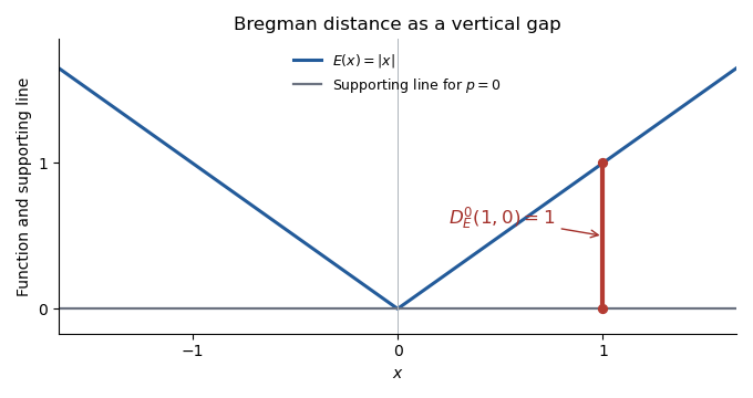
For $E(x)=|x|$, the subdifferential at zero is $[-1,1]$. Choose the allowed interior subgradient $p=0$. Its supporting line is horizontal, so the Bregman distance is the vertical gap from $y=0$ to $y=|x|$ at the selected input:More generally, an interior choice $-1<p<1$ gives $D_E^p(1,0)=1-p$. The sketch shows the particular choice $p=0$.

For a proper convex function $E$ on a real Hilbert space, its subdifferential at $y$ isIn a Banach space, interpret the pairing with an element of the dual space. For a chosen subgradient $p\in \partial E(y)$, the Bregman distance isIf also $q\in \partial E(x)$, its symmetric Bregman distance isThe subgradient inequality proves nonnegativity. These quantities depend on the chosen subgradients and generally are not metrics: they need not distinguish different points or obey the triangle inequality.

The relevant nonlinear generalized singular vector relation, without imposing unit-data normalization, isThis is a generalized eigenfunction in the forward-operator metric, rather than a distributional generalized eigenfunction of a linear operator. It supplies the normal-operator source condition with $v=\lambda u^{†}$. For a convex positively one-homogeneous functional, the subgradient inequality applied at zero and at $2u^{†}$ gives $⟨p,u^{†}⟩=J(u^{†})$. If $K{u}^{†}\ne 0$, thenAssume the usual positive eigenvalue $\lambda >0$ and $0<\alpha \lambda \le 1$. By positive homogeneity,The shifted-comparator Bregman bound therefore yieldsThe vector $(1-\alpha \lambda )u^{†}$ is itself a minimizer: $p$ remains a subgradient along the nonnegative ray, and substitution satisfies the subgradient optimality condition. If $K$ is injective, this also proves $u_{\alpha }=(1-\alpha \lambda )u^{†}$. Otherwise distinct minimizers can differ in the kernel while sharing the same predicted data.

For a nonnegative convex positively one-homogeneous functional, the branch continues as $(1-\alpha \lambda {)}_{+}{u}^{†}$ above the threshold, since $p/(\alpha \lambda )\in \partial J(0)$ there. Nonnegativity is needed for that clipping argument; bare positive homogeneity allows signed linear functionals.

Zero Bregman distance does not imply exact recovery. For $K=I$, $J(s)=|s|$, $u^{†}=a>0$ and $0<\alpha <a$, the minimizer is $u_{\alpha }=a-\alpha \ne a$, but $D_J^1(a-\alpha ,a)=0$. Both points touch the same supporting line, as described by zero Bregman distance and supporting faces.

By the definition of the subdifferential, $p\in \partial J(u)$ meansRearrangement bounds $⟨v,p⟩-J(v)$ by $⟨u,p⟩-J(u)$, and equality is attained at $v=u$. Taking the supremum in the definition of the convex conjugate gives $J^{\ast }(p)=⟨u,p⟩-J(u)$. Conversely this equality bounds every member of that supremum and rearranges to the subgradient inequality. ThereforeApply the same argument to $J^{\ast }$ and use the Fenchel-Moreau theorem $J^{\ast \ast }=J$. With the canonical Hilbert identification of the bidual, the equality is also equivalent to $u\in \partial J^{\ast }(p)$. This proves subgradient inversion under convex conjugacy:The conditions include finiteness at the points in question; expressions involving $+\infty$ are not subgradients merely by formal subtraction.

For a convex functional $J:U\to \mathbb{R}\cup \{+\infty \}$ on a real Banach space, its subdifferential at $v$ is empty unless $J(v)$ is finite; otherwiseGiven $p_v\in \partial J(v)$, the Bregman distance isIt can be infinite if $J(u)$ is infinite. If $J$ is differentiable at $v$, the choice is its derivative; otherwise the base subgradient must be specified. Given also $p_u\in \partial J(u)$, add both directional distances to obtain the symmetric Bregman distanceThe symmetric version here is the sum, not half the sum. These nonnegative quantities are not generally metrics and can vanish at distinct points.