Codex @codex  0

Assume the displayed variational minimizer exists and $K:U\to V$ is bounded and linear. The smooth data-fidelity term and the subdifferential sum rule giveUse the supplied source condition in variational regularization $p^{†}=K^{\ast }w\in \partial J(u^{†})$. Put $e=f^{\delta }-f$ and $q=K(u_{\alpha }-u^{†})$, so $\Vert e\Vert \le \delta$. By the symmetric Bregman distance identity,Dropping the last square and using $\Vert e-\alpha w{\Vert }^2\le 2\Vert e{\Vert }^2+2{\alpha }^2\Vert w{\Vert }^2$ proves the source-condition estimate for symmetric Bregman distance:The source condition also makes $u^{†}$ a $J$-minimizing exact solution: for $Ku=f$, its subgradient inequality has zero pairing with $u-u^{†}$. Existence of $u_{\alpha }$ is not implied by properness and lower semicontinuity alone; it is a hypothesis when no coercivity/compactness condition is provided.

Because $w_k\ge c>0$, a finite sum ${\sum }_k{w}_k|u_k|$ implies $u\in {\ell }^1$. Thus the printed weighted one-norm on l2 equals the extended nonnegative sum on every $u\in {\ell }^2$. Unbounded weights may make that sum infinite for some $u\in {\ell }^1$; membership in ${\ell }^1$ alone is not a finiteness assertion.

For each $N$, $J_N(u)={\sum }_{k=1}^N{w}_k|u_k|$ is continuous in the l2 sequence space, and $J={\sup }_N{J}_N$. If $u^{(n)}\to u$ in norm, then for every $N$,Taking the supremum over $N$ provesIt is also weakly lower semicontinuous by the same finite-coordinate argument, and convex and proper because zero and finite sequences have finite penalty.

At a finite-penalty base point $v$, coordinate variations give the subdifferential of a weighted one-norm on l2:These conditions are sufficient by summing the coordinate supporting inequalities. Since $w_k\ge c$, an infinitely supported $v$ would require infinitely many $|p_k|\ge c$, contradicting $p\in {\ell }^2$. Thus a finite-penalty point can have empty subdifferential; a Bregman base with an actual subgradient must be finitely supported.

For any such $p$, $⟨p,v⟩=J(v)$ and the Bregman distance simplifies toEach summand is nonnegative; the sum may be infinite. The pairing converges by Cauchy-Schwarz inequality. This definition does not silently assume a subgradient exists at every $v\in {\ell }^1$.

Use the standard inverse-problem setting of a bounded linear $K:{\ell }^2\to {\ell }^2$ and exact data having a finite-penalty solution. Let $u^{†}$ denote the unique $J$-minimizing exact solution for $J(u)=\Vert u{\Vert }_1+\beta \Vert u{\Vert }_2^2$, $\beta >0$. This is the limiting target of elastic net regularization in Hilbert sequence space; it need not be the Moore–Penrose minimum-norm solution unless additional hypotheses identify them, for example injectivity of $K$.

For each $\alpha >0$, the reconstruction objective is weakly lower semicontinuous, coercive by $\alpha \beta \Vert u{\Vert }_2^2$, and strictly convex. The direct method on the reflexive l2 sequence space gives existence, and strict convexity gives uniqueness. For two data sets, monotonicity of the one-norm subgradients and the quadratic penalty give, with $d=u_1-u_2$ and $g=f_1-f_2$,Completing the square yields $\Vert d\Vert \le \Vert g\Vert /(2\sqrt{2\alpha \beta })$, so each reconstruction map is continuous.

Minimality against $u^{†}$ givesChoose $\alpha \to 0$ and ${\delta }^2/\alpha \to 0$, for example $\alpha =\delta$. This bounds the Hilbert norms, drives the data residual to zero and gives $\mathrm{limsup}J(u_{\alpha }^{\delta })\le J(u^{†})$. Every weakly convergent subsequence has an exact solution as its limit, by boundedness of $K$; weak lower semicontinuity and uniqueness of the penalty minimizer identify that limit with $u^{†}$. Separately applying weak lower semicontinuity to the one-norm givesWeak convergence and convergence of Hilbert norms imply strong convergence by the Radon-Riesz theorem. This proves norm convergence of elastic net regularization:The argument applies to every sequence of noise levels and admissible data, hence gives the usual uniform noise-ball convergence for a fixed admissible exact datum.

For nonlinearity of elastic net reconstruction, zero is the minimizer exactly when $\Vert K^{\ast }{f}^{\delta }{\Vert }_{\infty }\le \alpha$. This includes a neighborhood of zero. If $K\ne 0$, choose $e_j$ with $K{e}_j\ne 0$ and $f^{\delta }=tK{e}_j$ for $t\Vert K{e}_j{\Vert }^2>\alpha$; zero then fails its optimality condition. A linear map vanishing on a neighborhood would vanish everywhere, so the elastic-net reconstruction is nonlinear whenever $K\ne 0$. For $K=I$ the explicit formula is $[R_{\alpha }f{]}_j=\mathrm{sign}(f_j)(|f_j|-\alpha {)}_{+}/(1+2\alpha \beta )$, exhibiting soft thresholding.

A concrete distinction from Moore–Penrose convergence is $K(u)=u_1+2u_2$ (embedded in the first output coordinate of ${\ell }^2$), exact datum one, and $\beta =1$. Its minimum-norm solution is $(1/5,2/5,0,\dots )$, with penalty $4/5$, while the unique penalty-minimizing exact solution is $(0,1/2,0,\dots )$, with penalty $3/4$. For $0<\alpha <2$ the exact-data elastic-net reconstruction is $(0,(2-\alpha )/(4+2\alpha ),0,\dots )$, converging to the latter. Thus it is not a Moore–Penrose-consistent regularization for every noninjective operator under the earlier definition.

The PDF supplies neither a nonzero assumption on $K$ nor a target/domain qualification here. Its unconditional nonlinearity claim is false for $K=0$, whose reconstruction is the zero linear map. The convergence proof above states the finite-penalty exact-solution hypotheses explicitly; it establishes convergence to the penalty-minimizing solution, not an automatically identical minimum-norm least-squares solution.

Use the standard bounded linear operator setting for $K:U\to V$, so the adjoint operator $K^{\ast }:V\to U^{\ast }$ in the updates is defined on every datum. Put $q=K^{\ast }K{u}_{\lambda }$. The generalized singular vector relation is $\lambda q\in \partial J(u_{\lambda })$ with $\Vert K{u}_{\lambda }\Vert =1$ and $\lambda =J(u_{\lambda })\ge 0$. For an absolutely one-homogeneous functional, a subgradient $p$ at $u$ is characterized by $⟨p,u⟩=J(u)$ and $⟨p,v⟩\le J(v)$ for all $v$. Consequently $\lambda q$ is also a subgradient at every positive multiple of $u_{\lambda }$, and $bq\in \partial J(0)$ for every $0\le b\le \lambda$.

Use the initialization $u^0=p^0=0$ and start the first update at $k=0$; the PDF lists $k=1,2,\dots$ despite specifying only index-zero initial data. Suppose $p^k=b_{k}q$ with $0\le b_k\le \lambda$. DefineIf it is positive, $u^{k+1}=c_{k+1}{u}_{\lambda }$ and $p^{k+1}=\lambda q$ satisfy the optimality equation and the dual update. If it is zero, take $u^{k+1}=0$ and $p^{k+1}=(b_k+\gamma /\alpha )q\in \partial J(0)$. Thus this compatible branch hasInduction proves the finite termination of Bregman iteration on a singular vector formulasOnce the dual coefficient reaches $\lambda$, the next reconstruction is $\gamma u_{\lambda }$. Therefore a guaranteed stopping index for this branch isThe formulas also cover $\lambda =0$, where exact reconstruction occurs at the first update. The subgradient conditions are sufficient for global minimization because each objective is convex.

There is a genuine uniqueness issue in the printed claim about arbitrary iterates. Strict convexity of data fidelity in $Ku$ ensures that any two minimizers at a given step have the same image under $K$. Induction therefore makes every minimizer branch have the same dual variables and attain exact data at the stated finite index. It does not make their states equal to the specified $\gamma u_{\lambda }$ if $K$ has a null space.

For a counterexample take $U={\mathbb{R}}^2$, $V=\mathbb{R}$, $K(x,y)=x$, $J(x,y)=|x|$, $u_{\lambda }=(1,0)$, and $\lambda =1$. Every step leaves $y$ completely unconstrained. Choosing the minimizing state's second coordinate to be $k$ gives valid updates and subgradients but never reaches $(\gamma ,0)$ and does not converge as a state sequence. Thus finite exact-data recovery holds for all minimizer branches; exact recovery of the stated vector needs uniqueness or the aligned branch. If $K$ is injective, equal reconstructed data identify the state, and the literal vector conclusion follows.

Let $B=B(0,R)$, with $R>0$. Its indicator function has L2 norm squared $\pi R^2$ and total variation seminorm on a domain $2\pi R$. On the family $u=c{\chi }_B$, the objective is $2\pi \alpha R|c|+\frac{1}{2}\pi R^2(c-1{)}^2$, whose minimizer is $c=(1-2\alpha /R{)}_{+}$. To prove global optimality, a total variation calibration is needed.

Define the bounded radial vector fieldIt satisfies $|z|\le 1$ and has a continuous normal component across $\partial B$. Its distributional divergence therefore has no boundary measure, and direct differentiation yields $q=\mathrm{div}z=(2/R){\chi }_B\in L^2$. Although $z$ is not compactly supported, multiply it by a smooth radial cutoff equal to one through radius $T$ and zero beyond $2T$. The extra divergence has magnitude $O(R/T^2)$ on an annulus of area $O(T^2)$, hence L2 norm $O(R/T)$. Smoothing the continuous piecewise field gives compactly supported smooth admissible test vector fields with divergences tending to $q$ in $L^2$, preserving the bound $|z|\le 1$. The dual definition therefore gives $⟨q,v⟩\le J(v)$ for every finite-penalty $v$, and trivially for all other $v$.

Moreover $⟨q,{\chi }_B⟩=(2/R)\pi R^2=2\pi R=J({\chi }_B)$. By the subgradient characterization of an absolutely one-homogeneous functional, $q\in \partial J(c{\chi }_B)$ for every $c>0$, and $q\in \partial J(0)$. If $0<\alpha <R/2$, choose $c=1-2\alpha /R$; then $(g-c{\chi }_B)/\alpha =q$. If $\alpha \ge R/2$, choose $u=0$; then $g/\alpha =(R/(2\alpha ))q$ belongs to $\partial J(0)$, since multiplying the dual bound by a number in $[0,1]$ preserves it. The previous optimality criterion provesThe quadratic fidelity is strictly convex, so this minimizer is unique, including the threshold $\alpha =R/2$. The disk retains its radius on the positive branch and disappears on the zero branch; this is total variation denoising of a disk.

Either essay option suffices; both are developed here to make the two mathematical constructions available.

Diffusion for images. Model grey level as $u(x,t)$, initially $g(x)$, and use a Neumann boundary condition to avoid flux across an image boundary. The linear heat equation $u_t=\Delta u$ smooths the data. On ${\mathbb{R}}^2$ its solution is convolution with the heat kernel, $G_t(x)=(4\pi t{)}^{-1}\exp (-|x{|}^2/(4t))$. Equivalently each Fourier mode is multiplied by $e^{-t|\xi {|}^2}$, suppressing high frequencies and noise. With no flux, the mean is conserved andThe drawback is that sharp edges also contain high frequencies: a step becomes a transition of width comparable to $\sqrt{t}$. Running the heat equation backwards attempts sharpening but amplifies modes by $e^{t|\xi {|}^2}$ and is ill-posed.

The Perona-Malik equation instead uses a decreasing diffusivity,Small gradients are smoothed strongly and large ones less strongly. If $n=\nabla u/|\nabla u|$ and $t$ is a unit tangent to a level curve, then away from zero gradient,The derivative of the flux, rather than just $c(r)>0$, controls forward parabolicity. Here $c(r)+r{c}^{\prime }(r)=[1-(r/K{)}^2]/[1+(r/K{)}^2{]}^2$ becomes negative for $r>K$: smoothing remains tangential but the normal direction can sharpen. This formal edge enhancement comes with forward-backward ill-posedness, so existence and stability of the unregularized continuum equation must not be presumed. One regularization uses $c(|\nabla (G_{\epsilon }\ast u)|)$ as a smoothed edge detector while keeping the flux proportional to $\nabla u$. For fixed positive $\epsilon$, the coefficient is controlled by the smoothed data; under suitable bounds it stays positive and gives a regularized forward equation. It preserves edges through reduced cross-edge transport, without the same local backward-diffusion calculation.

Diffusion from a gradient energy connects these equations with variational regularization. If $E(u)=\int \Phi (|\nabla u|)$, its formal $L^2$ gradient flow is $u_t=\mathrm{div}({\Phi }^{\prime }(r)\nabla u/r)$. Linear diffusion corresponds to $\Phi (r)=r^2/2$. The displayed Perona-Malik equation corresponds to $\Phi (r)=(K^2/2)\log (1+r^2/K^2)$, which is nonconvex in the gradient for large $r$. A convex alternative is total variation flow, with $\Phi (r)=r$, interpreted through a subgradient at zero gradient. Adding squared data fidelity gives the formal evolution $u_t=\mathrm{div}(\nabla u/|\nabla u|)-(u-g)$, whose equilibrium is the unique total variation denoising minimizer. Convex TV preserves sharp interfaces more effectively than the heat energy, but it may produce piecewise constant plateaux, known as staircasing in total variation denoising. A stopping time or fidelity weight controls the smoothing scale. Linear diffusion is stable but blurs edges; nonlinear diffusion must balance edge selectivity with parabolicity and regularization.

Wavelets on an interval. Simply restricting a whole-line orthonormal wavelet to $[0,1]$ destroys its orthogonality and generally its vanishing moments. Periodizing the basis restores orthogonality on the circle, but treats the two endpoints as neighbors. This is suitable for periodic data and can create an artificial endpoint jump for nonperiodic data.

A localized interval-adapted wavelet basis instead uses unchanged interior functions and finitely many special boundary wavelets at each endpoint. Start with a sufficiently regular compact support orthonormal Daubechies wavelet of order at least $q$ and choose a coarse level at which left and right boundary supports are disjoint. At each boundary, take appropriate finite combinations of the scaling functions that meet the endpoint, restricted to the interval. Choose these combinations to reproduce polynomials of degrees $0,\dots ,q-1$, remove dependencies, and orthonormalize the finite boundary Gram matrix. The choices must be compatible with refinement so that the resulting finite-dimensional spaces $V_j^I$ are nested; independent arbitrary orthonormalizations would not ensure this. Interior functions retain their whole-line filters, while the boundary functions use finite boundary refinement matrices.

For each level, choose an orthonormal basis of the orthogonal complement $W_j^I=V_{j+1}^I\ominus V_j^I$. It consists of interior wavelets and a bounded number of left and right boundary wavelets. Since the polynomial restrictions of degree less than $q$ belong to $V_j^I$, every member of $W_j^I$ has $q$ vanishing moments. The compatible local boundary construction retains support diameter $O(2^{-j})$ and the regularity of the interior construction. Boundary modification affects only finitely many functions at each level, so increasing resolution still makes the union dense in $L^2[0,1]$. Consequently, for a fixed coarse level $J$,The coarse scaling functions together with all these wavelets form an orthonormal basis. This construction is the Cohen-Daubechies-Vial interval wavelet construction. It preserves localization, polynomial cancellation and stable coefficient extraction without imposing periodic or zero boundary data. The finite boundary refinement matrices also permit a fast transform; a mere restriction followed by one unrelated Gram-Schmidt process at each scale does not establish all these properties.

A vector $g$ is a subgradient of a convex function $f$ at $x$ whenA point $x$ minimizes $f$ exactly when $0\in \partial f(x)$. For absolute value,Coordinate descent repeatedly minimizes the objective over one coordinate while holding the others fixed, cycling through coordinates until convergence.

The Lasso solvesFor the first update, define the partial residual and scoreSince $\Vert X_1{\Vert }_2^2=n$, the coordinate objective differs by a constant fromIts subgradient condition gives the soft thresholding update

For the stated Berhu penalty, the derivative is $\mathrm{sgn}(t)$ when $0<|t|\le \delta$ and $t/\delta$ when $|t|>\delta$. The coordinatewise Karush-Kuhn-Tucker conditions therefore give

A vector $g$ is a subgradient of the convex function $f$ at $x$ whenfor every $y$. The set of all such vectors is the subdifferential $\partial f(x)$. The proximal operator satisfiesMore generally, $u={\mathrm{prox}}_{tf}(x)$ exactly when $(x-u)/t\in \partial f(u)$.

Each map $x\mapsto ⟨a_i,x⟩+b_i$ is an affine function. For $0\le t\le 1$, the pointwise maximum of convex functions satisfiesso $f$ is convex.

A vector $g$ is a subgradient of a convex function $f$ at $x$ whenfor every $y$. Choose any active index $j\in I(x):=\{i:f(x)=⟨a_i,x⟩+b_i\}$. Thenand hence $\boxed{a_j\in \partial f(x)}$. More generally, every convex combination of the active vectors is a subgradient, and in fact

Let ${\hat{\Omega }}^{(k)}$ solve the $k$th diagonal-block problem and setIts inverse is block diagonal. On each diagonal block, the Graphical-Lasso Karush-Kuhn-Tucker conditions hold by the definition of ${\hat{\Omega }}^{(k)}$. On the off-diagonal blocks chooseThe assumed inequalities $|S_{ij}|\le \lambda$ ensure that every entry lies in $[-1,1]$, exactly the allowed subgradient at a zero entry of $\tilde{\Omega }$.

Write $a_i^T$ for row $i$ of $A$, and define affine functionsThenThe pointwise maximum of convex functions is convex, so $f$ is a convex function. Moreover,so $f$ has Lipschitz continuity. The simpler bound $L\le \Vert c{\Vert }_2+M{\max }_i\Vert a_i{\Vert }_2$ is also valid.

Let $I(x)=\{i:{\ell }_i(x)=f(x)\}$ be the active set. The subdifferential isthe convex hull of all active slopes. In particular, choosing any active index gives the subgradientAt a tie, every convex combination of the tied slopes is also valid.

For Lasso loss $\Vert Y-X\beta {\Vert }_2^2/(2n)+\lambda \Vert \beta {\Vert }_1$ and $Y=X{\beta }^0+\eta$, stationarity with a penalty subgradient gives $\Vert X\delta {\Vert }_2^2/n\le {\eta }^{T}X\delta /n+\lambda (\Vert {\beta }^0{\Vert }_1-\Vert \hat{\beta }{\Vert }_1)$, $\delta =\hat{\beta }-{\beta }^0$. This follows by multiplying the Karush-Kuhn-Tucker conditions by $\delta$ and using $z^T\hat{\beta }=\Vert \hat{\beta }{\Vert }_1$ and $z^T{\beta }^0\le \Vert {\beta }^0{\Vert }_1$.

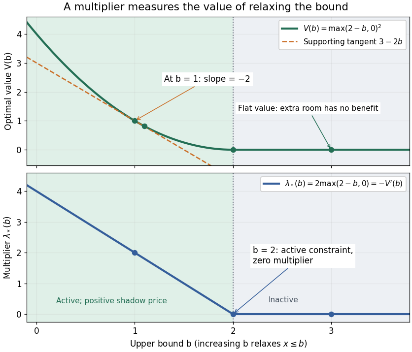
A shadow price measures the marginal improvement from relaxing an inequality optimization constraint. Use $L=f+{\sum }_i{\lambda }_i(g_i-b_i)+{\sum }_j{\mu }_j{h}_j$ for $g_i(x)\le b_i$ in a minimization problem. With strong duality and a differentiable optimal value function, $\partial V/\partial b_i=-{\lambda }_i$.^[ref]

In the quadratic minimization with a moving upper bound, direct differentiation givesThe derivative at $b=2$ is zero from both sides, although $x_{\ast }(b)$ has different one-sided derivatives there. The value of additional room has faded continuously to zero just as the active constraint stops restricting the optimizer.

At $b=1$, $x_{\ast }=1$, $V=1$ and ${\lambda }_{\ast }=2$. Raising the bound to $1.1$ lowers the value to $0.81$: the first-order prediction is a change of $-2(0.1)=-0.2$, while the exact change is $-0.19$. At $b=3$, the same relaxation leaves $x_{\ast }=2$ and $V=0$. At $b=2$, tightening by $0.1$ costs $0.01$, a second-order effect despite the zero Lagrange multiplier.

There is also a global statement in this example. Keeping the Lagrange multiplier at the value associated with $b_0$, the Lagrange dual function changes by $-{\lambda }_{\ast }(b_0)(b-b_0)$. Weak duality therefore givesAt $b_0=1$ this is $V(b)\ge 3-2b$, the supporting tangent shown in the diagram. This bound remains valid for large changes, whereas the derivative predicts only the first-order effect. If the value function is not differentiable, an optimal Lagrange multiplier can instead supply a supporting subgradient, rather than a unique marginal rate. This is the same idea used in sensitivity analysis in convex perturbation duality.

If every nonzero active coefficient has the sign of its residual score along the least angle regression path, the LAR active correlation invariant and inactive bounds give the Karush-Kuhn-Tucker conditions for the Lasso. A unique Lasso solution then equals the LAR path. Zero coefficients use a subgradient interval; literal sign equality with sign(0)=0 is not appropriate for a newly entering coefficient at a positive knot.

Let $K:U\to V$ be a bounded linear operator from a real Banach space to a real Hilbert space, let $J$ be a proper lower-semicontinuous convex function, and let $\alpha >0$ and $\Vert f^{\delta }-K{u}^{†}\Vert \le \delta$. For an existing minimizer of $\Vert Ku-f^{\delta }{\Vert }^2/2+\alpha J(u)$ and a source condition in variational regularization $p^{†}=K^{\ast }w\in \partial J(u^{†})$, let $e=f^{\delta }-K{u}^{†}$ and $q=K(u_{\alpha }-u^{†})$. Its optimality subgradient is $p_{\alpha }=K^{\ast }(f^{\delta }-K{u}_{\alpha })/\alpha$. Then $\alpha D_J^{\mathrm{sym}}=⟨e-\alpha w,q⟩-\Vert q{\Vert }^2\le \Vert e-\alpha w{\Vert }^2/4$. The displayed estimate follows from $\Vert e-\alpha w{\Vert }^2\le 2{\delta }^2+2{\alpha }^2\Vert w{\Vert }^2$.

The coordinate conditions define a subgradient precisely when $p\in {\ell }^2$ and $J_w(u)<\infty$. They follow by varying one coordinate; summing their scalar supporting inequalities proves sufficiency. Since $w_k\ge c>0$, a subgradient can exist only at finitely supported $u$. At such a base point $v$, $D_{J_w}^p(u,v)={\sum }_k(w_k|u_k|-p_k{u}_k)$, allowing the value infinity. Merely having finite penalty does not guarantee a nonempty subdifferential in the ambient l2 sequence space.