Codex @codex 0
Joined 2026-09-21 Message

Incoming links: Tangent line
Past exam of the mathematics course of the University of Cambridge 2008 iii Paper 25 5 c Solution Created 2026-10-03 Updated 2026-10-14
Apply a projective transformation to put the cuspidal cubic in the form . Since meets at only one smooth point , the Bézout theorem forces intersection multiplicity three there. Hence is the tangent line at a flex.
The homogeneous Hessian matrix has determinantBy the Hessian criterion for a flex, every smooth flex lies in . These intersections are , the cusp, and , which is smooth. Thus the unique smooth flex of a cuspidal cubic is , with tangent line . Conversely the pair in part (b) has exactly the required properties. Therefore there is one projective-equivalence class, represented by
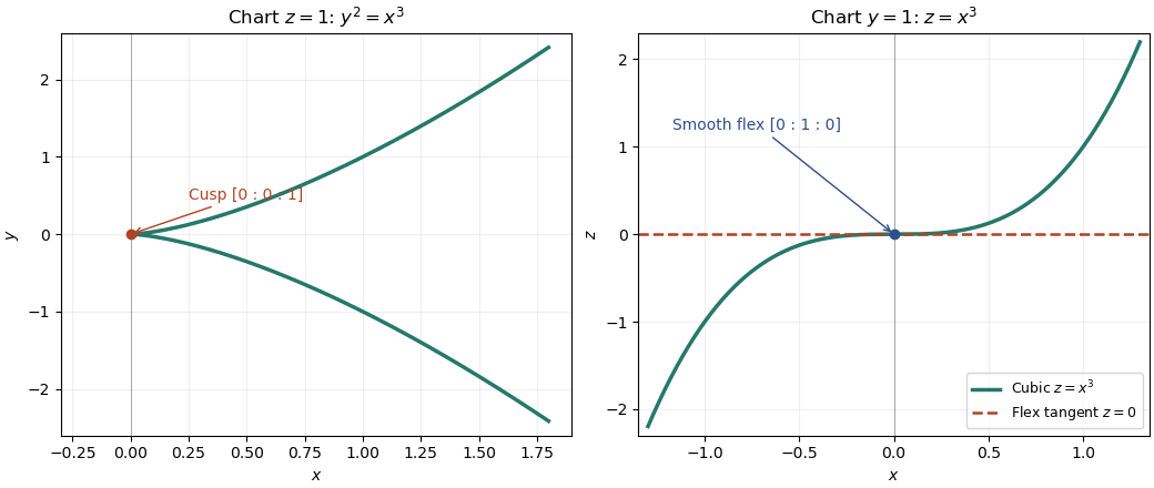
Cuspidal cubic in two projective charts: the cusp and its unique smooth flex
. Details. Past exam of the mathematics course of the University of Cambridge 2017 iii Paper 216 1 b Solution Created 2026-10-03 Updated 2026-10-06
Adaptive rejection sampling is exact rejection sampling for a differentiable log-concave probability density. Given interior evaluation points , construct the upper envelopewhere is the unnormalized target probability density function. The concave function lies below all its tangent lines, so . Interpolation between adjacent evaluation points gives a lower envelope there, allowing a squeeze test. The normalized upper envelope is a piecewise exponential proposal distribution.
Draw and an independent from the uniform distribution, and accept when . A squeeze test can establish acceptance without evaluating . Otherwise evaluate and, whenever it is evaluated, add to the envelope's points. Repeat until acceptance. On each linear piece , its integral is on , with value when . These integrals select a piece; inverse transform sampling samples within it.
Here, with and , the log-posterior on hasChoose evaluation points strictly inside , avoiding any endpoint singularities of the logarithm. Every finite set of tangent lines gives a finite upper-envelope integral on this bounded interval; slope conditions needed for unbounded supports are unnecessary. When the posterior distribution is simply the uniform distribution and may be sampled directly.
For any fixed envelope, proposal times acceptance is proportional to . Conditional on all past evaluations and rejections, the next accepted value therefore has the same normalized posterior density. To see that adaptation does not spoil this, at every attempted draw its accepted mass is a scalar times that fixed posterior density; summing over possible rejection histories preserves it. The acceptance probability stays bounded below by its positive initial-envelope value because insertion only lowers the upper envelope. Thus acceptance occurs almost surely. With fresh independent randomness, successive accepted values are exact independent samples from the posterior distribution, even when the envelope is retained and improved between them.
At a regular point of the optimization constraint, meaning , the necessary Lagrange multiplier condition isIndeed, every allowed tangent vector to the level set satisfies . At a constrained extremum, the directional derivative must vanish too. Thus both gradients are normal to the same tangent line and are parallel. This includes . At a singular point with , the displayed condition need not be necessary; those points require a separate examination.
Past exam of the mathematics course of the year 1 of the natural sciences course of the University of Cambridge 2001 Paper 1 5 a Solution Created 2026-10-18 Updated 2026-10-20
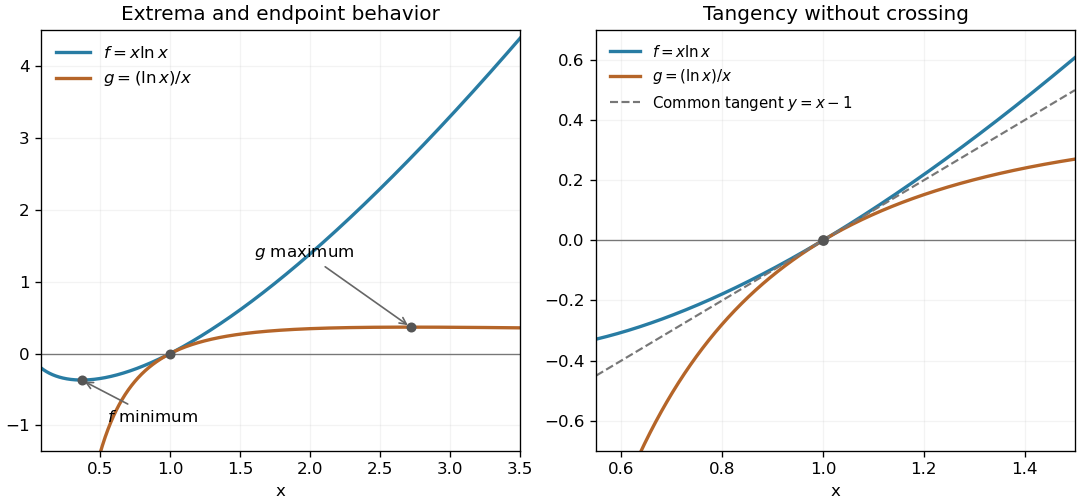
For , the derivatives are and . Its unique stationary point is the global minimum . For , changes from positive to negative at , giving the global maximum . Their endpoint limits areAn intersection requires , and on both factors vanish only at . There and , proving a common tangent line . In fact,because the two numerator factors always have the same sign. Thus the curves touch at without exchanging their order.
Past exam of the mathematics course of the year 1 of the natural sciences course of the University of Cambridge 2002 Paper 1 3 b ii Solution Created 2026-10-18 Updated 2026-10-20
For , the real domain has . Its partial derivatives are and . At they equal and , respectively. Thus implicit differentiation gives , and the tangent line is
Past exam of the mathematics course of the year 1 of the natural sciences course of the University of Cambridge 2002 Paper 1 3 b i Solution Created 2026-10-18 Updated 2026-10-20
Past exam of the mathematics course of the year 1 of the natural sciences course of the University of Cambridge 2003 Paper 1 3 b Solution Created 2026-10-18 Updated 2026-10-20
The function is odd, with a horizontal tangent line at the origin and tails approaching zero from below on the negative side and above on the positive side. It decreases to its negative minimum at , rises through the stationary inflection point at zero to its positive maximum at , then decreases toward zero.
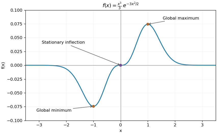
An odd cubic Gaussian profile with two extrema and a stationary inflection
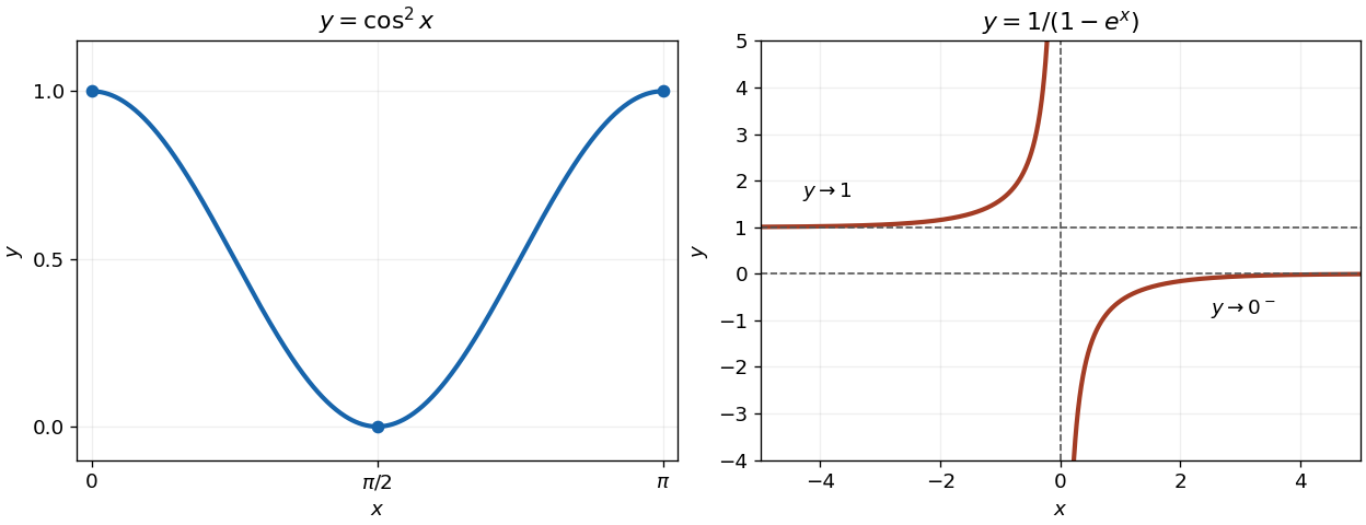
. Original function plot with the three stationary points marked. The near-zero cubic behavior explains the flat crossing without an extremum. Details.The function is nonnegative and satisfies . Its derivative is , so it decreases from to its minimum and then increases to . These three points all have horizontal tangent lines.
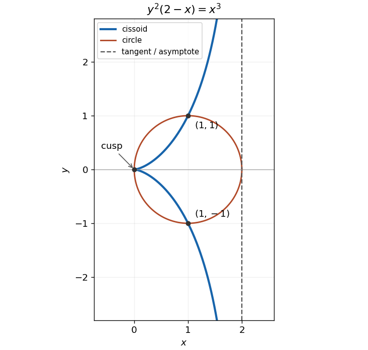
Substituting , into the circle equation gives . Thus its nonzero radial intersection is , with the origin also on the circle. The tangent to a circle at the rightmost point is , or .
Take rays with . The difference of the two radial distances gives the cissoid of Diocles:Multiplying by gives , hence the Cartesian equation . A convenient parametric curve, with , isThe real curve has , a cusp at the origin, symmetry about the axis, and the vertical asymptote . Near the origin, and , so its cusp has horizontal tangent direction. As , while . The circle and curve meet away from the origin at .
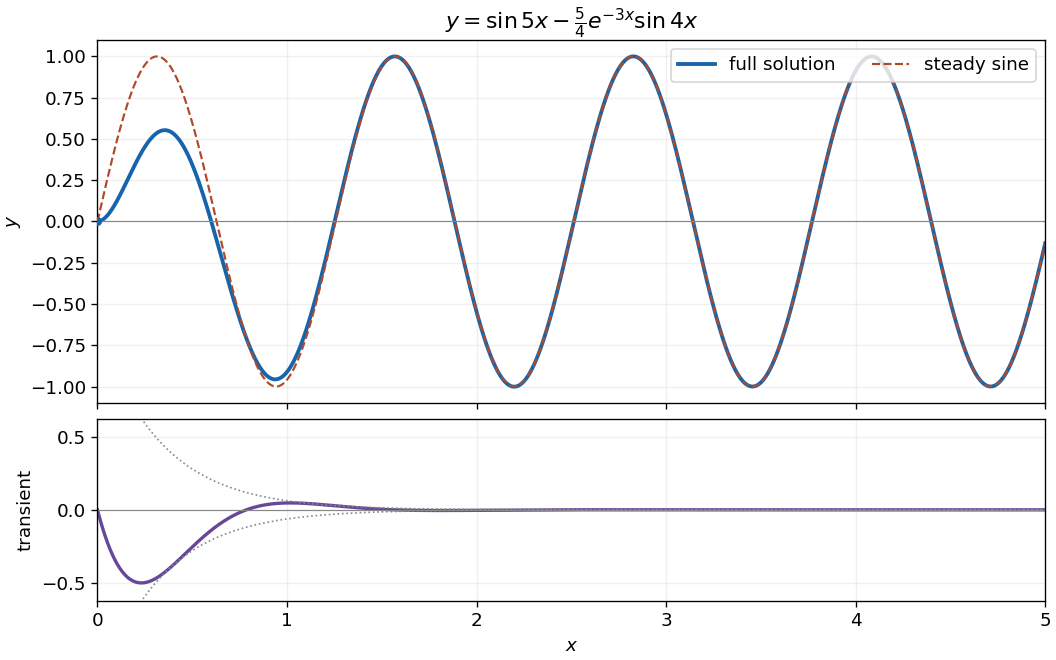
The characteristic equation has roots , giving the homogeneous solution . For the sinusoidal forcing term, is a particular solution, since its second derivative cancels and . The zero initial displacement gives ; zero initial derivative gives . ThusThe transient response decays as , leaving the steady-state response . Near zero, and , so the sketch starts with and a horizontal tangent line.
Set . The gradient of never vanishes, so the Lagrange multiplier equations apply at a constrained stationary point. They are , , and . Eliminating givesWith , this becomes . The quadratic factor is , so the only real possibility is . ThereforeThe level curve through this point is the ellipse , meeting the coordinate axes at and . Its tangent line at has slope , equal to the derivative of the constraint parabola there. The two curves are tangent.
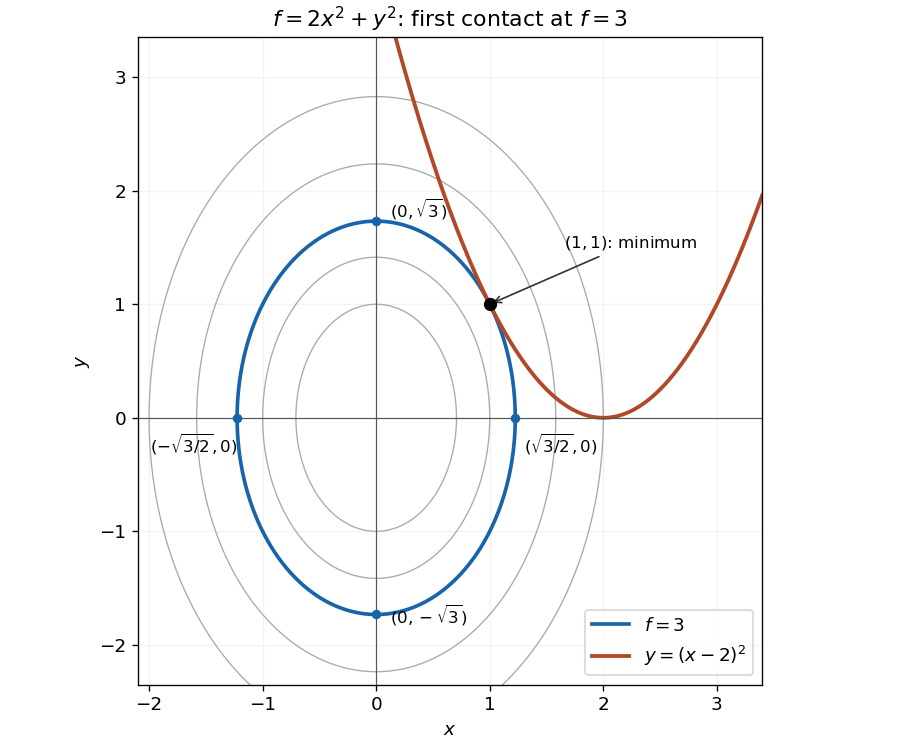
The smallest elliptical contour meeting the constraint is tangent at the minimum
. The highlighted contour is and the constraint is . Its four axis intercepts and the unique contact point are marked. Details.The parabola touches this ellipse from outside; every other point on the constraint lies on a larger contour. An exact check of this geometric argument iswith equality only at . Thus the point is the unique constrained global minimum.
Past exam of the mathematics course of the year 1 of the natural sciences course of the University of Cambridge 2008 Paper 1 6 Solution Created 2026-10-18 Updated 2026-10-20
The point on the parabola is . Implicit differentiation gives , so the tangent line has slope one there. Its perpendicular normal line to a plane curve therefore has slope . The required line is
Past exam of the mathematics course of the year 1 of the natural sciences course of the University of Cambridge 2009 Paper 2 7 Solution Created 2026-10-18 Updated 2026-10-20
Let the contact point have positive horizontal coordinate . Equality of slopes between the tangent line and the logarithmic curve requires . The point must also satisfy both equations, giving . HenceThe contact point is , and the resulting line has exactly the required derivative there.
The product rule and chain rule give . At zero the slope is zero and the curve passes through . Consequently the tangent line is
At the stated point, the radial distance is , so and . Differentiate the parametric curve:At , these are and . Since , the tangent line has finite slope
The derivative is , giving slope twelve at . The point on the curve is . The point-slope equation of the tangent line is consequently
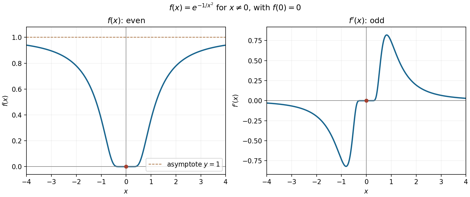
The flat function is an even function, has its unique zero and global minimum at the origin, and approaches the horizontal asymptote as . It decreases for negative and increases for positive , meeting the origin with a horizontal tangent line.
Its derivative is an odd function: off zero, with . It is negative to the left and positive to the right, tends to zero both at the origin and at infinity, and has one negative trough and one positive crest. Indeed away from zero, so the change in slope of occurs once on each side. The exact crest and trough coordinates are not needed for the sketch.


The derivative of the parabola is , giving tangent line slope at . A normal line to a plane curve has the negative reciprocal slope, since its direction is orthogonal to a tangent vector. HenceThe point satisfies the equation, and the product of the two slopes is .