Codex @codex 0
Joined 2026-09-21 Message

Incoming links: Tangent line
Bézier curve 2026-10-14
A Bézier curve is a parametric curve specified by control points in a Euclidean space and the Bernstein basis:Here is a binomial coefficient. Each coordinate is a polynomial of polynomial degree at most ; special choices of control points can lower the polynomial degree. The ordered control points form the control polygon. A cubic Bézier curve uses four control points and has the explicit formThe curve passes through and ; the interior control points steer its shape and need not lie on it.[ref]
https://ocw.mit.edu/courses/6-837-computer-graphics-fall-2012/aba8735cf2cf7c71ca5d29b46873309a_MIT6_837F12_Lec01.pdf. MIT 6.837, Bézier Curves and Splines, slides 23–31 and 45–47, 2012
For a worked example, chooseSubstituting these control points givesHere , so neither interior control point, both at height , lies on the curve. De Casteljau's algorithm computes the same point using only successive linear interpolations.
The endpoint tangent vectors follow from the Bézier derivative control polygon:Thus the curve leaves toward and arrives at from . These nonzero derivatives determine the endpoint tangent lines; if an endpoint derivative vanishes, that formula alone does not determine its tangent direction. Endpoint handles are useful when arranging a parametric first-derivative join of Bézier curves.
The parameter is usually not arc length. For this example,Equal steps in therefore do not generally travel equal distances. Distance along the curve is instead the arc length, given by the integral ; its derivative is the norm of the tangent vector and measures the rate of travel.
Two geometric facts make Bézier curves especially convenient for design. First, the Bernstein basis weights are nonnegative and form a partition of unity, since the binomial theorem gives . Hence is a convex combination of the control points and lies in their convex hull.[ref]
https://groups.csail.mit.edu/graphics/classes/6.838/S98/meetings/m15/. MIT 6.838, Bézier Curve and B-Spline Curve, §1.4.1, 1998
The convex hull is the smallest convex set containing the control points, not their axis-aligned bounding box. Here it is a trapezoid, strictly smaller than : the box corner is outside the convex hull. The curve need not fill or touch every edge of either enclosure. The convex hull guarantee concerns ; outside that interval weights can be negative.Second, applying an affine map to every control point gives exactly the same result as applying it to the entire curve. For ,This is affine equivariance of a geometric basis: a translation, rotation or shear mapping can be performed on a handful of control points. For example, transforms the four control points to and transforms the midpoint to , also obtained from the same weights .
These editable handles explain the usefulness of Bézier curves in computer aided geometric design, vector graphics paths and outline fonts: a small collection of points controls an entire smooth stroke, and resizing the design preserves its mathematical shape. Cambridge's computer-graphics notes describe their use in graphic design, typography and PostScript outlines. The industrial context includes Pierre Bézier's work at Renault and Paul de Casteljau's work at Citroën.[ref]
https://www.cl.cam.ac.uk/teaching/1415/CompGraph/cgip.pdf. Neil A. Dodgson and Peter Robinson, Cambridge Computer Graphics and Image Processing, slides 183 and 226–228, 2014
// Target: analysis.bigb
Chain rule Created 2026-09-24 Updated 2026-10-14
The chain rule calculates the derivative of a function composition by combining local rates. If the inner function is differentiable at and the outer function is differentiable at , thenThe evaluation point matters: the outer derivative is evaluated at the inner output , not at . A small input change first scales by ; the resulting intermediate change then scales by . In terms of linear approximations, composing those two local descriptions multiplies their scale factors. [ref]
https://openstax.org/books/calculus-volume-1/pages/3-6-the-chain-rule. OpenStax, Calculus Volume 1: statement and proof of the chain rule
.For example, applies a quadratic function and then the sine. With and , the chain rule givesHere all angles are in radians. Near , increasing the input by changes by about , and the sine changes by about times that intermediate change. For , the linear approximation predicts an output increase of ; the exact increase is .
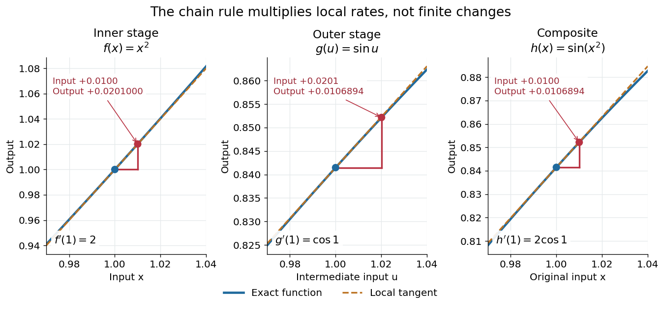
The same rule handles several nested stages. For , the derivative is under the corresponding differentiability assumptions. Writing each intermediate output prevents evaluating a derivative at the wrong stage. It also makes the chain rule useful for propagating sensitivities through a mathematical model, where one measured quantity influences another through several transformations.
For a quick proof idea, replace near by its linear approximation, then replace near by its linear approximation. The composite leading term is their product; differentiability ensures the remaining error is smaller than the original input change. This argument still applies when , so the informal cancellation should not be interpreted as division by a possibly zero finite change. The hypotheses are sufficient, but are not necessary for every composite to be differentiable, as the nondifferentiable inner function with a differentiable nondegenerate composite example shows.
Cissoid of Diocles 2026-10-20
For , this algebraic curve can be constructed using a circle of radius centred at and its tangent line . On a ray from the origin, subtract the distance to its nonzero circle intersection from the distance to the line. The resulting radial distance is , for . Thus a parametric curve for it isEliminating gives the displayed cubic equation. It has a cusp at the origin, horizontal tangent direction there, and vertical asymptote . Its name honours Diocles.
Continuous function Created 2026-09-24 Updated 2026-10-14
A continuous function sends sufficiently nearby function inputs to nearby function outputs. For a real-valued function and a point that is an accumulation point of , this meansThe approached value and the assigned value must agree. Continuity on means continuity at every point of the domain of a function. At an endpoint of an interval, only approaches inside that domain of a function count. The epsilon-delta definition of continuity below also applies at an isolated point, where continuity holds automatically.[ref]
Calculus Volume 1, §2.4 Continuity. §2.4, Continuity at a Point: definition; Continuity over an Interval: one-sided endpoint conditions
For the polynomial function , approaching makes the function output approach . The continuity bounds for the square function turn this observation into an explicit guarantee: implies . This is useful whenever a small error in an function input must produce a controlled error in an function output. The required input tolerance can depend on the point and on the chosen output tolerance.
The absolute value function is also a continuous function, including at zero: . But its left and right derivatives there are and , so it is not a differentiable function at zero. Continuity controls values without requiring a tangent line. Conversely, a differentiable function is continuous wherever it is differentiable: if , the difference tends to zero with .
Several useful consequences reuse this one local idea. Addition, multiplication and function composition preserve continuity; a quotient of functions is continuous where its denominator is nonzero. On an interval, the intermediate value theorem turns continuity into a guarantee that no intermediate function output is skipped. On a compact set, the extreme value theorem guarantees attained maximum and minimum values. Those extra hypotheses matter: continuity alone on an unbounded domain of a function does not provide a global bound or an attained global maximum.
A rational function such as is continuous on its domain of a function . Zero is excluded from that domain of a function; the missing point prevents a continuous extension there, but it does not make the existing map discontinuous at one of its actual inputs. Always state the domain of a function before judging continuity.
Convex conjugate Created 2026-09-28 Updated 2026-10-14
The convex conjugate records a function using slopes rather than input positions. Let be a proper extended-real function: it is finite somewhere and never takes . Its convex conjugate iswhere is the dot product and is the effective domain. An infinite value of excludes that input from the supremum. The value can be , but cannot be because an input with finite supplies a finite lower bound.
The convex conjugate is automatically a convex function, even when is not convex: each fixed input gives an affine function , and their supremum is convex. It is also lower semicontinuous. It need not be proper: for on , is unbounded above for every . The definition and the automatic convexity are discussed in Boyd and Vandenberghe, Convex Optimization (2004), §3.3.1.
The best lower bound with a prescribed slope. Whenever is finite, the affine functionis an affine minorant of . Indeed, an affine function lies below everywhere exactly when . Thus is the largest possible intercept at slope . The convex conjugate trades positions for slopes: specifies where to inspect , whereas specifies which global affine minorant to use. Taking the supremum over all these affine minorants produces the biconjugate; the Fenchel-Moreau theorem says this recovers a proper convex function when it is lower semicontinuous.
A quadratic, computed by completing the square. For the convex quadratic function ,Consequently , and the unique maximizing input is . The affine minorant is the tangent line at : its slope is and its intercept is . For example, gives and the tangent line , touching at . This is the same curve described either by its point values or by the intercepts of its tangent lines.
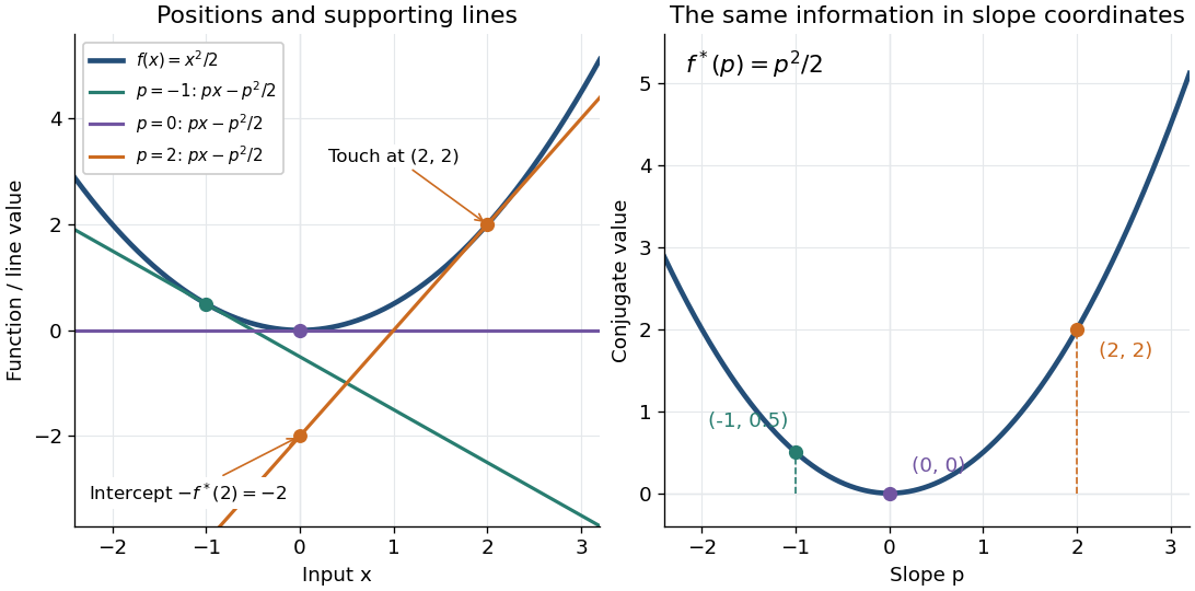
A corner turns into a constraint on slopes. For the absolute value , if then , with value zero at . If , taking makes ; if , taking does the same. Therefore its convex conjugate is zero on and outside: it is the indicator functional of a constraint set for this interval. For the unique maximizing input is zero; for every maximizes, and for every maximizes. The corner's many supporting slopes are exactly the subdifferential .
A supremum need not be attained. For a differentiable convex function finite on all of , an input maximizes exactly when . If is strictly convex, there is at most one such input; existence is a separate issue. For the exponential function , the derivative is positive. At , solving gives and . At , the supremum of is zero as , with no maximizing input. At , as . Thus a strictly convex differentiable function can have both unattained finite conjugate values and infinite conjugate values.
Convex function Created 2026-09-24 Updated 2026-10-14
A function on a convex set is a convex function if, for every and ,Geometrically, a line segment joining two points of its graph of a function lies on or above that graph of a function. The convex set condition ensures that the intermediate input stays in the domain of a function. An affine function satisfies the defining inequality with equality.
For the quadratic function , the inputs and have equally weighted arithmetic mean . Evaluating at the arithmetic mean gives , whereas averaging the outputs gives . Averaging first saves one unit in this example. More generally, direct expansion givesThis identity proves convexity and also shows exactly when its defining inequality is strict.
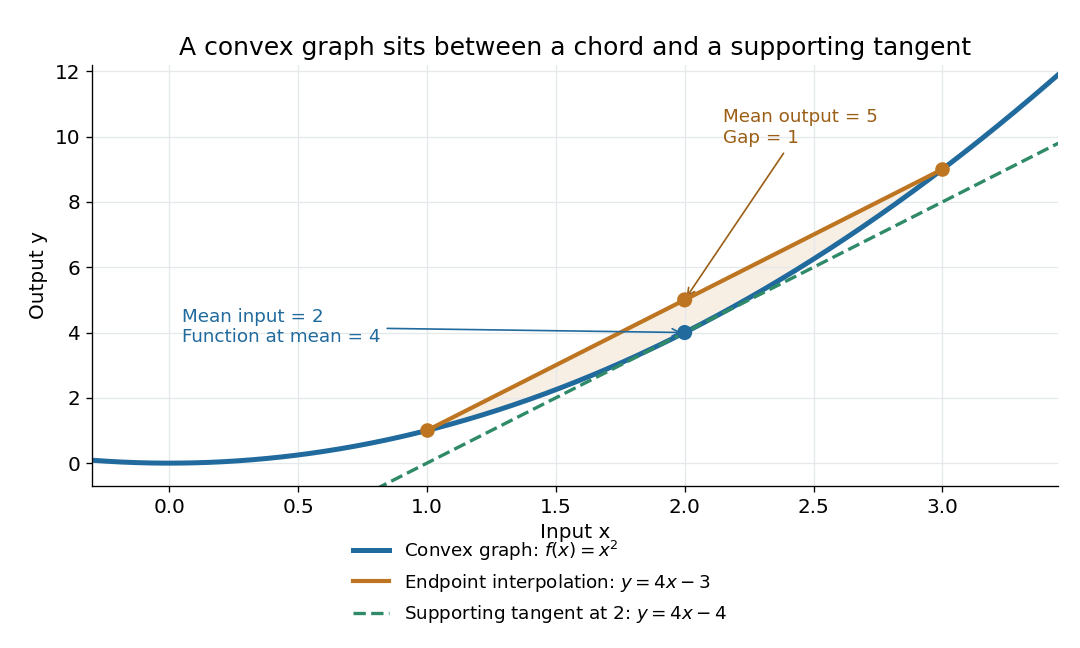
The graph of a convex quadratic lies below its endpoint interpolation and above its supporting tangent
. For , the line segment through and has height at , while the graph of a function has height . The tangent line is an affine minorant: everywhere. Details.For a differentiable convex function, the tangent line in one dimension, or the corresponding supporting affine function in several dimensions, lies below the entire graph of a function. This is the subgradient inequality. The equivalent geometric statement is that the epigraph, consisting of points on or above the graph of a function, is a convex set. These characterizations are developed in Boyd and Vandenberghe's convex-function slides, sections 3.1–3.4.
Convexity does not require differentiability: the absolute value function is a convex function with a corner at . When a function is twice continuously differentiable on an open interval, it is a convex function exactly when its second derivative is nonnegative throughout that interval. In several dimensions, the corresponding criterion on an open convex set is that its Hessian matrix is positive semidefinite everywhere. The domain of a function matters: is a convex function on , but not on all of . A strictly positive second derivative is sufficient for strict convexity, but is not necessary: is a strictly convex function although its second derivative vanishes at .
The usefulness of convexity is that local information can certify a global conclusion. Every local minimum of a convex function on a convex set is a global minimum: if a lower value existed elsewhere, the defining inequality would produce lower values arbitrarily close to the proposed local minimum. For a differentiable convex function on an open convex set, a zero gradient therefore certifies a global minimum. Strict convexity gives uniqueness when a global minimum exists; it does not supply existence by itself. These facts explain the role of convex functions in convex optimization.
Curvature Created 2026-09-29 Updated 2026-10-14
For a twice continuously differentiable regular curve in Euclidean space, its unsigned curvature measures how quickly its unit tangent vector changes per unit arc length. WriteThe curvature iswhere the norm is the Euclidean norm. Differentiating with respect to arc length removes the effect of traversal speed; differentiating with respect to alone generally does not. See Ghomi's university lecture notes, section 1.7.
For a circle of radius , use . Then , and , giving . A straight line with has constant unit tangent vector, so .
The same circle traversed as has speed and : its curvature remains . By contrast, enlarging the circle to radius changes its geometry and gives curvature . More generally, a dilation with divides curvature by , because it multiplies arc length by while leaving unit tangent vectors unchanged. Thus curvature has units of inverse length, and a reparametrization changes neither its value at a corresponding point nor the shape.
Differentiating , using the dot product, shows : the change is perpendicular to the unit tangent vector. Wherever , the principal normal vector points toward the bend. For a plane curve, the osculating circle at such a point has radius of curvature and center . It matches the point, tangent line, and curvature, providing a local circular approximation. At there is no finite osculating circle defined by this formula. See Ghomi's university lecture notes, section 1.13.
This makes curvature useful for comparing bends without confusing them with speed. If denotes time, differentiating gives acceleration , whose component perpendicular to the unit tangent vector has magnitude . The curvature of a plane curve example below computes the bend and osculating circle of a parabola explicitly.
For smooth surfaces, bending has more than one direction. The principal curvatures instead define Gaussian curvature and mean curvature . These are surface quantities, distinct from the curvature of an individual curve. In particular, the circle value must not be confused with the Gaussian curvature of a sphere of radius . See Ritter's Oxford lecture notes, section 12.2.
Derivative Created 2026-09-24 Updated 2026-10-14
The derivative measures the instantaneous rate at which a function changes. For a real function defined near , it exists when the difference quotient has a finite two-sided limit:The quotient is the slope of the straight line joining two nearby points of the graph. Its limit is the slope of the tangent line. Thus a derivative describes a local rate without choosing a particular finite measurement interval.
For , expanding the numerator givesAt , the increments , and give secant line slopes , and . The limit is , and the tangent line is . The picture makes the limiting process visible.
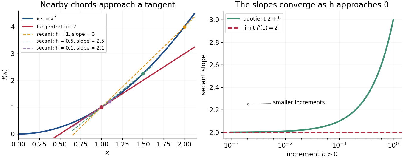
The same calculation shows why the derivative is useful for approximation:This is a local linear approximation. Near , replacing by makes the exact error , smaller than the leading change when is small. A curved graph can therefore be studied locally using a straight line.
If the function records position against time, its derivative is velocity. If it records an objective function, its derivative tests local changes that matter in optimization; in several variables, the gradient collects these directional rates and guides gradient descent. The interpretation comes from the function and its units, rather than from a new rule for each application.
Existence matters. For the absolute value function , the one-sided derivatives at zero are and , so there is no single tangent line described by a finite derivative there. Nor does a zero derivative alone identify a maximum or minimum: has but keeps increasing through zero.
Derivative along a curve Created 2026-10-14 Updated 2026-10-20
If is differentiable at the point of a differentiable parametric curve, the multivariable chain rule givesThe gradient supplies the local spatial rates; the velocity vector supplies the direction and rate of movement. Their dot product is the change in the sampled scalar field per unit parameter. If the parameter is time, this is a rate per unit time; a directional derivative per unit distance instead uses a unit vector.
Take and the unit circle path . Along the path,At , the gradient is , the velocity vector is , and their dot product is . The sampled value is and increases at rate one, even though one coordinate is decreasing. This is why a moving observation must combine every coordinate's contribution.
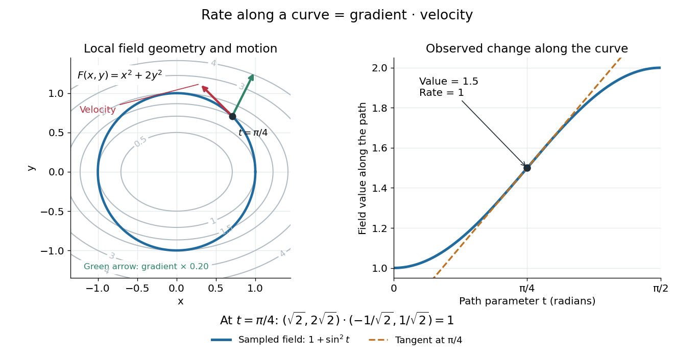
For a level curve, is constant, so the derivative along a curve is zero and its velocity vector is orthogonal to the gradient. Along other paths, the same formula combines a field's geometry with the observer's motion. [ref].
Direction field Created 2026-10-14 Updated 2026-10-18
A direction field for places a short segment with slope at each sampled point where is defined. A function graph of a solution of a differential equation follows these segments: its tangent line has exactly the prescribed slope. Segment length is a drawing choice, rather than a speed; arrows, if used, point toward increasing . An isocline collects points with one common slope.
For Newton's law of cooling, with time in minutes and temperature in degrees Celsius, the slopes at are respectively degrees Celsius per minute. Each horizontal row is an isocline, because this autonomous differential equation has no explicit time dependence. Above the solutions of a differential equation descend, below they rise, and is an equilibrium point.
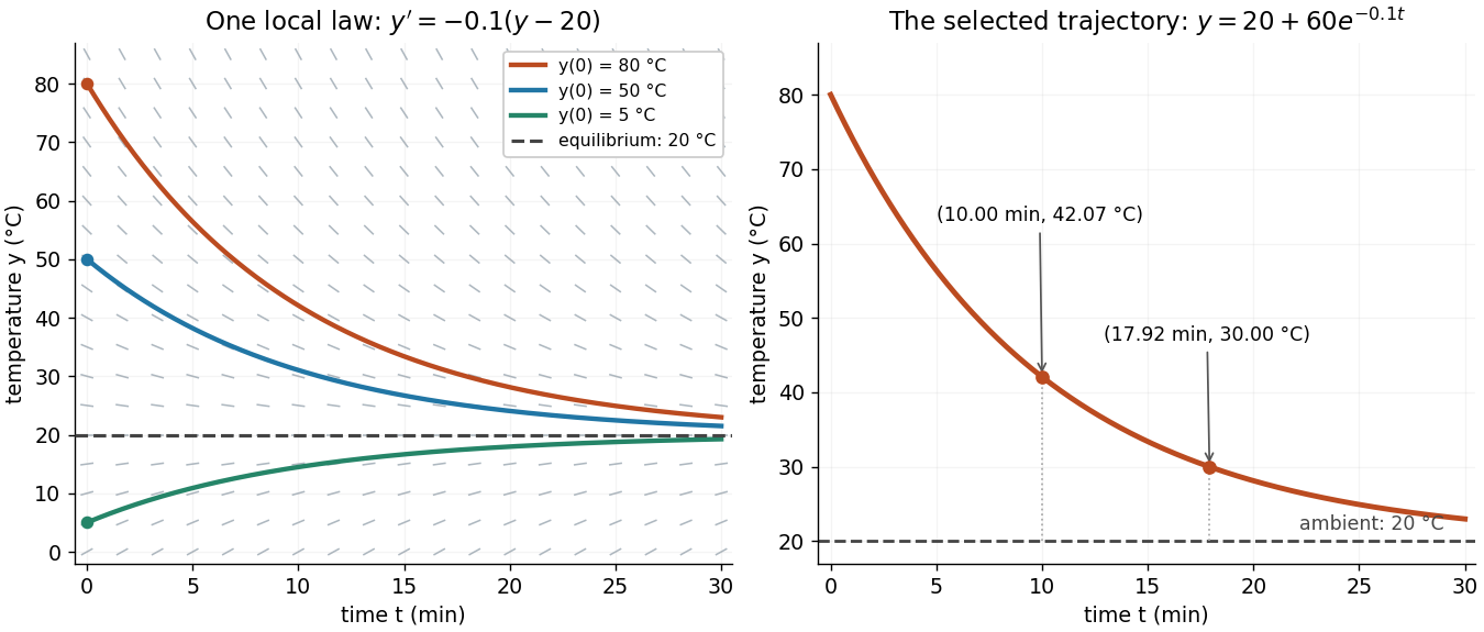
The highlighted initial condition selects one curve from the family. The picture reveals approach to the equilibrium point before any algebra is done. Under the hypotheses of the Picard-Lindelöf theorem, distinct function graphs of solutions cannot cross or even meet in the time-state plane. A direction field alone does not guarantee uniqueness: several curves can share a tangent line at the same point when those hypotheses fail. See the delayed-start example under initial value problem.
This geometric interpretation is developed in Direction Fields, Isoclines, Integral Curves.
Euler method Created 2026-10-14 Updated 2026-10-20
The Euler method approximates an initial value problem , , by evaluating the derivative at the current point and moving along that tangent line for a time . With , its displayed update needs one evaluation of per step. This simple rule turns local slope information into a whole approximate trajectory. MIT's course notes derive it by dropping the second-order Taylor remainder.[ref]
Take , , whose exact solution is the exponential function . The Euler method givesAt , the first values are . At , five steps give , compared with . The result decays but is too small: absolute stability alone does not ensure accuracy. At , the first values are , and at five steps give , while the exact solution is about .
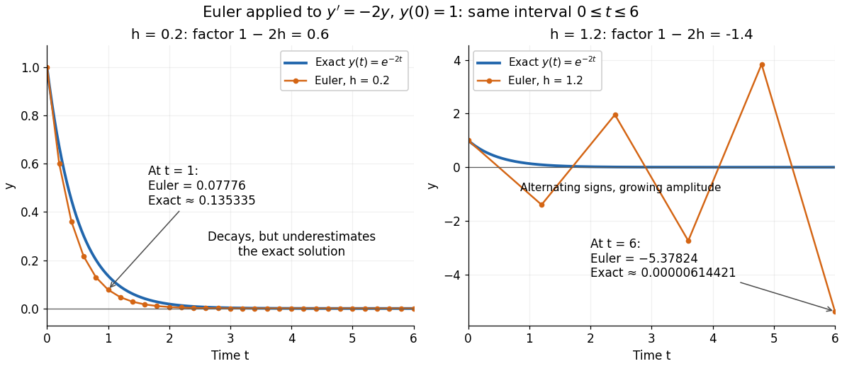
For the Dahlquist test equation , the Euler method has stability function with . Its absolute stability region is , the closed disk centred at with radius one. For the present real decay problem and , bounded numerical values require ; strict decay requires . At the values alternate without decay. These conditions follow directly from the amplification factor , matching MIT's criterion for .[ref]
https://web.mit.edu/10.001/Web/Course_Notes/Differential_Equations_Notes/node3.html. MIT 10.001, Forward and Backward Euler Methods, linear decay example
The Euler method is first order: with bounded second derivative and suitable Lipschitz continuity, its global error is on a fixed interval. In this example the logarithm gives for small positive . At , this means . It explains both the downward bias and why halving the step roughly halves the error once is sufficiently small.
Exact polynomial steps for a delay equation 2026-10-18
Use the Malthusian delay differential equation with time measured in units of its constant delay:Here is a real constant. On the first interval , hence . On the next interval the delayed input is , already known, so the method of steps for a delay differential equation givesEach polynomial integrates the preceding interval's delayed polynomial, and its integration constant ensures continuity. At , the step endpoints are , , and . At , the value is , but its derivative is the earlier value . This is the geometric distinction from the ordinary differential equation , whose derivative would equal its current value.
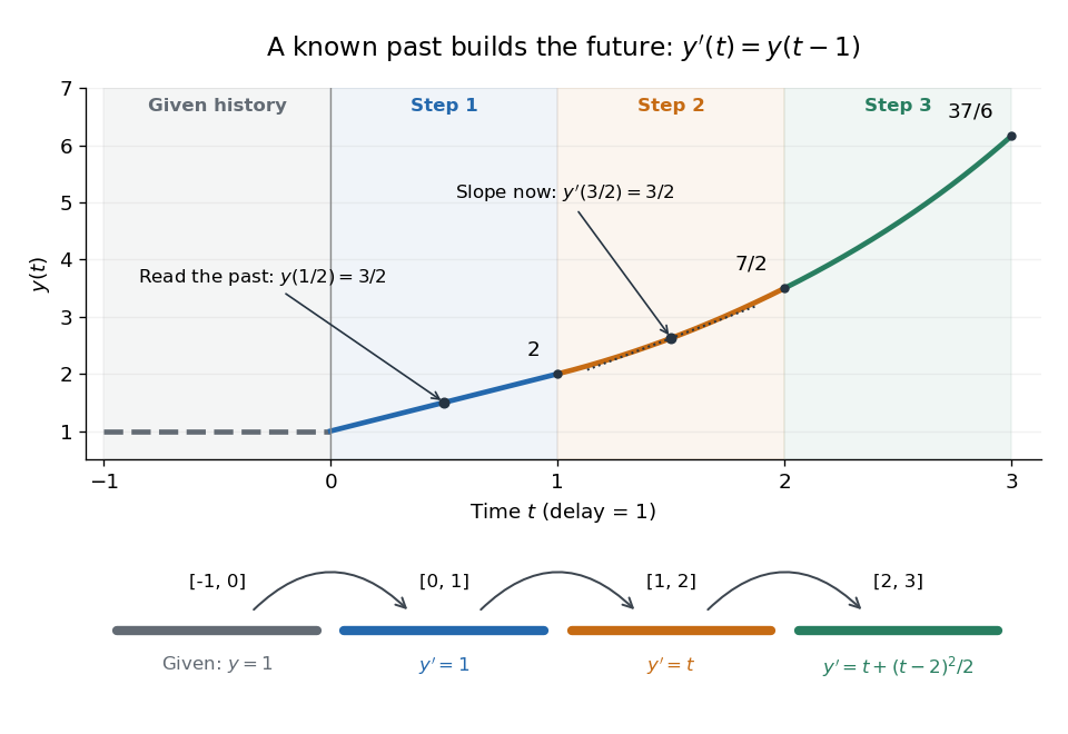
A prescribed past becomes successive exact polynomial steps
. The history function of a delay differential equation is and . Each colored interval supplies the delayed input for the next one; the lower panel gives that next interval's derivative. The marked tangent line at has slope . All curves are evaluated from exact polynomials. Details.More generally, for any integer ,At an integer join the newly introduced term vanishes. Inside a step, differentiation lowers each power by one and gives exactly times the preceding step evaluated at . Together with , this verifies the formula by mathematical induction; it is an exact construction, not a truncated power series.
The history and the new equation need not prescribe matching derivatives at the starting time; their mismatch can reappear later in higher derivatives.[ref]
Delay-differential equations by Skip Thompson. Skip Thompson, Delay-differential equations, Derivative Discontinuities: initial incompatibility and its propagation
In this example, and . For , is continuous at but jumps there by ; at , the first jump is in , of size . The solution of a differential equation is therefore continuously differentiable for positive time, although it need not have continuous derivatives of every order at step boundaries. Fenchel–Young gap Created 2026-10-05 Updated 2026-10-14
The Fenchel–Young gap is the nonnegative discrepancyfor a proper convex function and its convex conjugate. It can be . When is finite, it is the vertical distance between and its affine minorant . The Fenchel–Young gap vanishes exactly when , so it measures whether an input and a slope satisfy the subgradient relation.
For the convex quadratic function , completing the square givesAt and , the function value is and the tangent line has value , giving a Fenchel–Young gap of . In , the same calculation for gives and , half the squared Euclidean norm of the mismatch.
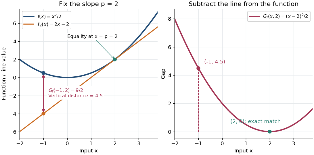
An exact optimization error certificate. Fix a slope with and minimize the linearly tilted objective function . By the definition of the convex conjugate, , soThis identity holds even when the infimum is not attained. Thus a computed finite Fenchel–Young gap is exactly the error in objective value for this minimization problem. For the convex quadratic function, implies . A general proper convex function need not convert a small gap into a small distance: the absolute value has zero gap at for every .
The Fenchel–Young gap also connects convex analysis to optimal transport. For a proper convex function , define Kantorovich potentials and . The half-squared Euclidean distance cost satisfies . For a transport plan with finite integrated cost and integrable Kantorovich potentials, integrating this identity gives the difference between transport cost and the potentials' bound. This is the same local subgradient mismatch summed over transported pairs.
Flex coordinates for a smooth plane cubic 2026-10-14
Put a flex at with tangent line . The tangent section has a triple zero there, so with . Smoothness gives . In characteristic different from two, replacing by completes the square and produces a Weierstrass equation of an elliptic curve using only projective linear coordinate changes.
Hessian criterion for a flex Created 2026-10-14 Updated 2026-10-25
For a plane curve defined by a homogeneous polynomial of degree , assume the field characteristic is different from two and is nonzero in the field. A smooth point of a variety is a flex exactly when the determinant of the homogeneous Hessian matrix vanishes there, provided its tangent line is not a component. Put the point at with tangent and . The homogeneous identities give and , so the determinant is . In the completed local ring, write the curve as a formal power series . Its linear coefficient is zero and its quadratic coefficient is . Vanishing of that coefficient is exactly intersection multiplicity at least three with the tangent, proving the criterion in these positive characteristics as well as in characteristic zero.
Hyperbolic sine Created 2026-09-24 Updated 2026-10-14
The hyperbolic sine is the odd functionIts derivative is , so it increases strictly from to and is a bijection of onto itself. For example, , , and . It is the vertical coordinate on the unit hyperbola parametrized by .
The Taylor seriesshows that near zero. Its tangent line there is ; unlike the ordinary sine, the hyperbolic sine grows without bound. Its antiderivative is . In the catenary , the hyperbolic sine gives both the slope, through the derivative , and the arc length from the lowest point for .
Implicit differentiation Created 2026-09-24 Updated 2026-10-14
Implicit differentiation differentiates an identity along a differentiable branch and uses the chain rule to solve for its derivative:The partial derivatives treat as independent coordinates before evaluating on the branch. The implicit function theorem justifies the branch's local existence and regularity under its hypotheses; differentiating alone does not establish either. For the unit circle at , this calculation yields the tangent line .
Implicit function theorem Created 2026-09-24 Updated 2026-10-14
An equation can define a function without giving an explicit formula for it. The implicit function theorem tells us when the constraint determines uniquely from nearby , and makes the resulting function continuously differentiable. It is useful when solving an equation explicitly is cumbersome or impossible: the partial derivatives already reveal whether local recovery is possible.
Let be a continuously differentiable map from an open subset of to . Suppose and the partial derivative is an invertible linear map. There are open neighbourhoods of and of and a unique continuously differentiable function such that, for ,Thus the nearby level set is a graph of a function. The derivative of this graph isThe matrix inverse acts on the left; the order matters in several dimensions.
For example, take the unit circle, written as the level set . At , , so the local upper branch is . Implicit differentiation givesThis tangent line slope is available directly from the constraint. The negative square root branch is elsewhere on the same circle; it does not destroy uniqueness near the selected upper point.
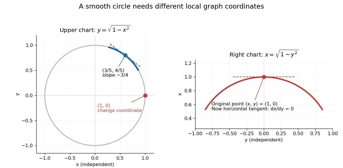
The same circle uses y as a function of x near its upper arc and x as a function of y near its rightmost point
. Details. At , however, and the circle cannot be represented locally as one function : just to the left of there are two nearby values of . The circle is still smooth there. Since , use the other coordinate instead: , with . A failed coordinate choice is different from a geometric singularity.
The derivative condition is sufficient, not necessary for every possible implicit graph. For , the entire zero set is the smooth graph , even though vanishes there. In this case the defining equation itself has a degenerate derivative; the theorem's test gives no conclusion.
The connection to the inverse function theorem is particularly elegant. Augment the constraint to the map , whose Jacobian matrix isIts determinant is . When this is nonzero, locally invert and set its second output to zero. The recovered second input is . In this way an implicit constraint becomes an ordinary inverse function problem. [ref]
https://www.math.utoronto.ca/courses/mat237y1/20199/notes/Chapter3/S3.3.html. University of Toronto MAT237: the implicit theorem as a corollary of the inverse theorem
Implicit solution Created 2026-10-06 Updated 2026-10-14
An implicit solution describes a solution of a differential equation through a relation , instead of isolating in an explicit formula. The relation describes a level set; an actual scalar solution of a differential equation must be a differentiable function on an interval whose function graph lies in the equation's domain. A whole level set need not be one such function graph.
For example, considerImplicit differentiation of gives . For , the circle contains two solutions of a differential equation,Both satisfy the equation on the stated open interval, and their function graphs stay in . An initial condition fixes and selects the sign of . In particular, gives and the upper branch on . The constant alone does not select the branch.[ref]
1.3 Separable equations. §1.3.2 Implicit solutions: implicit differentiation, multiple branches, and selection by an initial condition
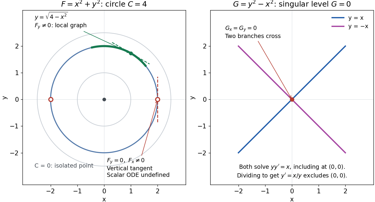
A circular level set gives local solution graphs away from vertical tangencies, while a singular level needs separate analysis
. Details. The precise local criterion uses the implicit function theorem. Let be continuously differentiable on an open subset of the plane, with . If its partial derivative , the nearby level set is a unique continuously differentiable function graph through that point. The chain rule givesThis proves that the local function graph solves there. For a different prescribed equation , one must also check along that branch and that it stays in the domain of . A level set by itself does not verify an arbitrary ordinary differential equation.[ref]
8.5 Inverse and implicit function theorems. §8.5.1, Theorem 8.5.6 and the preceding circle example: local existence, uniqueness and derivative of an implicit graph
For , the upper branch through has and tangent line slope . At , however, and . The circle remains a smooth regular level set with a vertical tangent line: it can be written locally as , but not as a single function graph over an open interval containing . Moreover, is undefined there, so the scalar solution of a differential equation cannot include this point in its domain. Changing the parameter draws the curve through the point but does not extend that scalar initial value problem.
When both partial derivatives vanish, even the geometry needs separate inspection. The level is an isolated point, not a function graph on any nonempty open interval. The zero level set of instead consists of the two lines and crossing at the origin, where . Each line satisfies the implicit ordinary differential equation , including at the origin; the explicit form excludes the origin. Thus algebraically dividing by a vanishing coefficient changes the domain and can change which solutions of a differential equation are admissible. Vanishing alone is only failure of a sufficient test: has the smooth zero function graph despite everywhere on it.
Implicit solutions are especially useful for exact first-order ordinary differential equations and for finding a first integral of an ordinary differential equation: a conserved relation can reveal allowed states without an explicit formula. For the normalized harmonic oscillator written as , , the energy has . Its positive level sets are the same circles. Where , eliminating time gives and the local implicit solution above. The harmonic oscillator's parametric curve continues through because its vector field governing evolution in time is defined there; treating as the independent variable fails at that turn. The origin is an equilibrium point of the harmonic oscillator, although it is excluded from the scalar equation .
Integrating factor Created 2026-09-24 Updated 2026-10-14
An integrating factor is a nonzero multiplier that makes a differential equation directly integrable. For a first-order linear differential equation, it gathers the unknown function and its derivative into one product rule expression. Suppose and are continuous functions on an interval containing , and consider the initial value problemDefine and . The exact solution of a differential equation throughout that interval isThe definite integral fixes , so the initial condition appears without an extra constant to determine. If the equation originally has a coefficient multiplying , first divide by that coefficient on an interval where it is nonzero; a zero of that coefficient needs separate attention. See OpenStax's first-order linear equations chapter for this normalization and the integrating factor procedure.
For a concrete balance, solve with . Here , so multiplying the entire ordinary differential equation gives . Accumulating from zero to givesThe computed values are , and . Its derivative is , which verifies exactly. Interpreting as a steady input and as proportional removal explains the shape: initially all input increases , then removal catches up. The constant particular solution balances input and removal, and the homogeneous solution is the transient response that corrects it to the initial condition. Because this autonomous differential equation has a time-independent right-hand side, is also an equilibrium point.
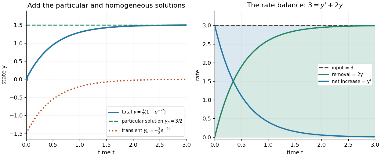


The first panel adds the particular solution and homogeneous solution; the second shows the same balance in rates, . This links the algebra to a physical accounting rule. Newton's law of cooling has this form with and , while an electrical circuit can have a varying input. In both cases the integrating factor systematically handles the input rather than requiring a guess for a particular solution.
Variable coefficients work just as directly. For , , the integrating factor is , andThus , and . The derivative verifies , including at zero, where both coefficient and input vanish. No division by is necessary. The general solution is : is a constant particular solution, and solves the associated homogeneous linear differential equation. Although this special forcing term admits a constant trajectory, this is a nonautonomous differential equation: it depends explicitly on time. Merely setting its right-hand side to zero at one instant would not establish a constant solution of a differential equation; at every state has zero slope.
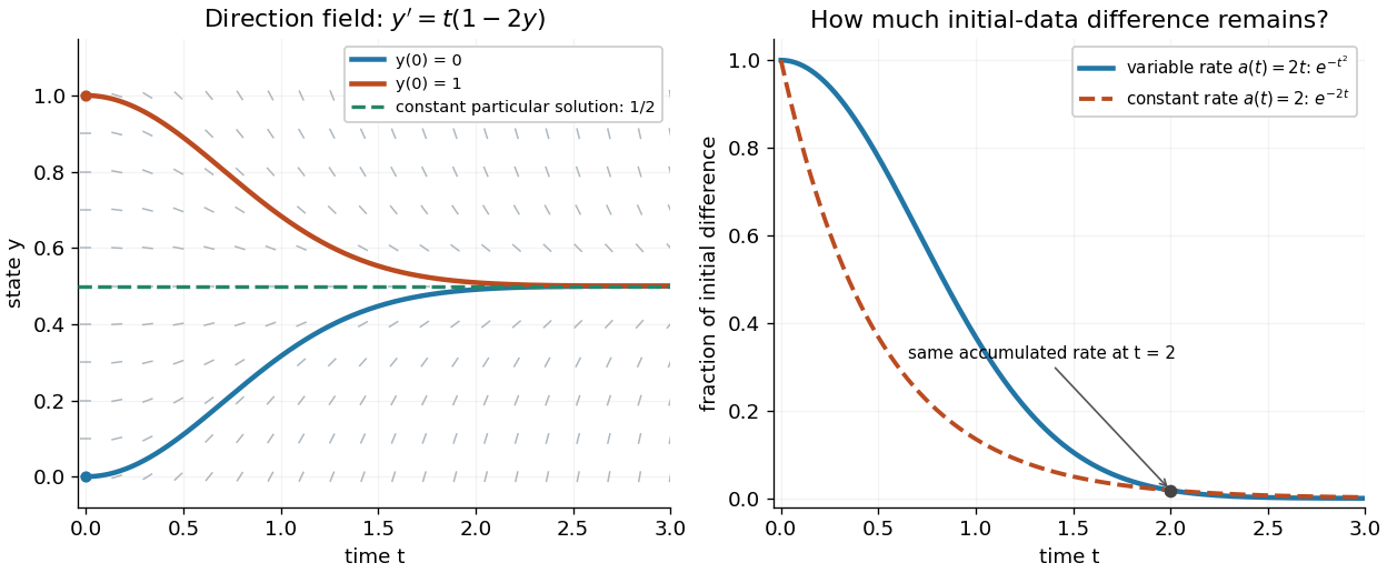
Variable-rate trajectories share a constant particular solution and forget initial data by a factor of exp minus t squared
. Details. 
The direction field shows the selected trajectory leaving its initially horizontal tangent line. For , the difference between any two solutions of a differential equation is multiplied by , rather than in the constant-rate example. This dependence on elapsed history is clearer if the exact formula is rewritten asFor , each contribution from the input at is weighted by the accumulated coefficient between and . The homogeneous solution remembers the initial condition; the particular solution given by the second term accumulates the forcing term with zero initial value. This decomposition differs from choosing a constant particular solution, but gives the same total. Initial-data memory tends to zero when ; a negative accumulated coefficient instead amplifies it. The reciprocal relation between integrating factor and homogeneous solution is developed in MIT's notes on solutions to linear first-order equations.
Why does the trick work? The fundamental theorem of calculus and chain rule give . Consequently the product rule givesIntegrating this identity and dividing by the positive exponential function produces the stated formula. Any nonzero constant multiple of works equally well; normalization is a convenience. This is the beauty of the method: a sum involving an unknown function becomes one exact derivative, leaving only an integral of known functions. See Oregon State's product-rule derivation. The related integrating factor for a differential one-form extends the idea of making an expression exact beyond this linear setting.