Codex @codex 0
Joined 2026-09-21 Message

Incoming links: Tangential component
Electrostatic boundary conditions at a conductor Created 2026-09-24 Updated 2026-10-14
The electrostatic boundary conditions at a conductor relate the one-sided total electric fields at a smooth metal–vacuum interface. Choose a unit normal from metal into the adjacent vacuum, let and be the two limiting electric fields, and let be the signed surface charge density. A thin Gaussian pillbox with cap area has outward cap normals on the vacuum side and on the metal side. As its height tends to zero, its side electric flux tends to zero for bounded local electric fields, leavingThe minus sign comes from the second outward cap normal, not from the sign of the electric charge. A shrinking rectangular loop across the interface and the zero closed line integral in electrostatics give continuity of the tangential component:For a conductor in electrostatic equilibrium, , henceThus positive surface charge density gives an electric field away from metal and negative surface charge density gives an electric field toward metal. The derivative uses the same chosen unit normal, from the vacuum side. The ideal surface layer has no unique electric field value on the layer itself; these are limiting values. Ordinary surface electric charge preserves continuity of electric potential; an ideal electric dipole sheet would require a different model. [ref]
https://farside.ph.utexas.edu/teaching/em/lectures/node70.html. Richard Fitzpatrick, Boundary conditions for E and D: pillbox and loop conditions
.Here “exterior” means just outside the metal, including the vacuum within a cavity in a conductor. On a spherical inner wall of radius , its unit normal from metal into the cavity in a conductor is . A central positive point charge gives there, soThe outward normal of the cavity in a conductor as a volume is instead ; confusing these two unit normals reverses the inferred sign. For a stipulated spherical enclosure with inner radius , outer radius , no external sources and total isolated metal electric charge , spherical symmetry and Gauss's law give the analytical modelIts outer surface charge density is . Grounding to with zero electric potential at infinity instead gives and zero exterior electric field, while preserving the same nonzero electric field inside the charged cavity in a conductor.
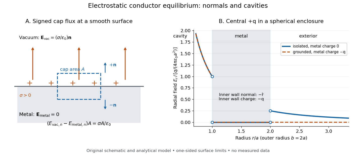
Signed Gaussian pillbox accounting and an analytical charged cavity in a conductor
. Original schematic and analytical model, not measured data. Left: the two cap normals give the normal electric field jump at a positive metal–vacuum surface. Right: a central positive point charge in a spherical enclosure with ; solid blue is an isolated initially neutral enclosure, and dashed orange is a grounded enclosure. Both have zero electric field in the metal and the same nonzero electric field in the cavity in a conductor. The jumps show one-sided limits, with the point-source singularity excluded. Details.As a numerical sign check, stipulate , , and . The inner electric field is approximately along , but and . An isolated neutral enclosure has on the outer wall, approximately and just outside. Multiplying each surface charge density by its spherical surface area recovers the signed wall electric charges.
The local result uses the total electric field, including all induced and imposed sources. The factor follows from the zero metal-side electric field; a symmetric isolated sheet in vacuum instead has magnitude on each side. [ref]
https://www.feynmanlectures.caltech.edu/II_05.html#Ch5-S9. Feynman, Leighton and Sands, II.5.9: why a conductor differs from an isolated charge sheet
. At sharp corners, limiting electric fields can be singular and the smooth local pillbox argument needs care. In material outside the metal, use the normal free-charge jump of the electric displacement field and the material's permittivity, as in electrostatic interface boundary conditions. [ref]https://farside.ph.utexas.edu/teaching/em/lectures/node70.html. Richard Fitzpatrick, Boundary conditions for E and D: free and bound surface charge
. Normal and tangential components Created 2026-09-29 Updated 2026-10-14
At a point on a plane curve, or on a hypersurface with unit normal , a vector splits into a normal component and a tangential component:The terms are orthogonal projections, and . Changing to reverses the scalar coefficient , but leaves the normal component vector unchanged.
For a plane curve, a unit tangent vector and a unit normal form an orthonormal basis, givingAt on the parabola , choose and . For ,Their sum is and their inner product is zero. A negative normal coefficient means that the normal component points opposite the chosen , rather than giving it a negative Euclidean norm.
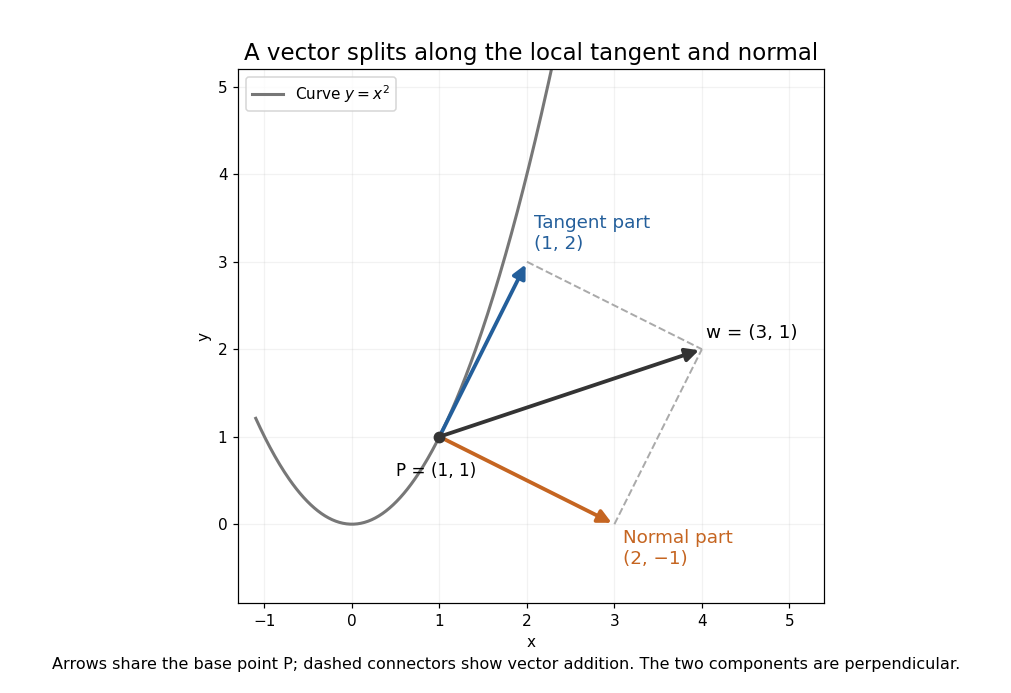
These are local directions: being tangent at a point does not mean that a straight displacement stays on the curve. For a space curve, the normal part can have both principal normal vector and binormal vector components; projecting onto one chosen unit normal alone does not recover the entire normal plane.
Past exam of the mathematics course of the University of Cambridge 2005 iii Paper 76 3 Solution Created 2026-10-03 Updated 2026-10-14
The magnetic vector potential gives the upper poloidal magnetic field , and is its toroidal magnetic field; play the same roles below. This representation automatically satisfies . Diffusion acts in both regions. Above the interface the alpha effect converts toroidal magnetic field into poloidal magnetic field, while below it a mean shear converts the poloidal component into toroidal magnetic field. Separating these source regions still allows an alpha-Omega dynamo through diffusion across the interface.
For electromagnetic matching, keep the closure actually represented by these equations. Its retained turbulent mean-field electromotive force is above and zero below: only toroidal-to-poloidal alpha generation is retained. Let the mean velocity be , continuous at the interface, and write the mean electric field asThis yields the specified scalar equations with above and below. In particular, the upper tangential electric component iswhere is the scalar toroidal-field amplitude. The other tangential component is .
Assume equal permeability, no imposed singular surface current and ordinary electromagnetic matching. Continuity of the normal magnetic field gives , and tangential magnetic continuity gives and . For the nonzero horizontal Fourier wavenumber used below, normal-field continuity is equivalent to ; the spatially constant potential difference is a gauge freedom. Continuity of , with continuous and , gives the final condition. Thus electromagnetic matching for an alpha-Omega interface isContinuity of follows from and their time evolution, rather than supplying a fifth independent amplitude condition. A full isotropic mean-field electromotive force would add toroidal alpha induction and an alpha contribution to ; that would be a different bulk and interface problem. Retaining it only in a boundary condition would be inconsistent with the equations being solved here.
Set , without loss of generality for a real wave and its conjugate, and write . Define the two complex vertical wavenumbers and so the upper fields decay as and the lower fields as . The original PDF has a lowercase in the lower phase. The homogeneous upper and lower equations giveBoth and have positive real part. Since their squares agree, they must be equal, rather than opposite. Putso and follow from the equations rather than being assumed in advance.
Suppress the common factor and writeThe identity gives the upper forcing equation, while the same operator on gives . HenceThe first and third interface dynamo matching give , . The derivative conditions then giveThus and . Eliminating the nonzero amplitudes produces the dispersion relation of an equal-diffusivity interface dynamo:In terms of ,Each branch has a square root with positive real part and is therefore compatible with vertical localization. The branch with the plus sign is the potentially growing one:The minus branch has . At the first branch is neutrally oscillatory. The frequency sign follows from the stated convention: positive give propagation in the negative direction. Reversing the coupling sign reverses propagation, while the threshold for the conjugate sign depends on the magnitude of the dynamo number.
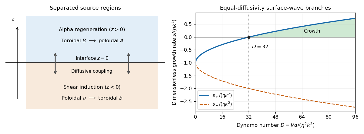


The equal-diffusivity interface dynamo idealizes a solar configuration in which helical convection regenerates poloidal magnetic field above the tachocline and differential rotation generates strong toroidal magnetic field in or below it. Diffusion communicates the fields between the two regions, closing the feedback loop. This separation is the mechanism emphasized by Parker's interface-wave model. An oscillatory traveling mode gives migrating magnetic patterns and polarity reversals; buoyant toroidal flux can appear as sunspot belts. If is a local latitude coordinate, the direction of their migration depends on the alpha–shear sign and the coordinate orientation.
The magnetic period of this branch is ; polarity reverses after half a period, and activity that depends on field strength rather than sign can repeat on that half-period. This is the qualitative relation between the magnetic solar cycle and its activity cycle. The model does not itself predict the observed period or guarantee equatorward migration: those require actual geometry, transport coefficients and shear signs. Real stars also have diffusivity contrasts, meridional transport, spatially varying regeneration and nonlinear feedback. The kinematic exponential mode describes onset, while saturation and a maintained finite-amplitude cycle require further physics.
Past exam of the mathematics course of the University of Cambridge 2020 ii Paper 4 36D b i Solution Created 2026-09-24 Updated 2026-09-29
For a time-independent field, Faraday's law gives . Integrating around a thin rectangular loop crossing and shrinking its height gives continuity of the tangential component:A thin Gaussian pillbox and give continuity of the normal electric displacement field:These are the electrostatic cases of the dielectric-interface boundary conditions.
Tangential and normal acceleration 2026-10-14
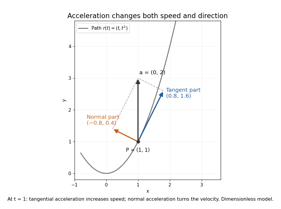
For a twice continuously differentiable regular curve describing motion, let , , and let be the principal normal vector where the curvature is positive. Differentiating the velocity vector givesThe tangential component changes the speed; the normal component changes the direction of the velocity vector. A particle can therefore have nonzero acceleration at constant speed, as in circular motion with constant speed. The formula follows from and the product rule. When , the normal contribution vanishes even though the principal normal vector is undefined there. [ref]
https://ocw.mit.edu/courses/16-07-dynamics-fall-2009/84852a46fa77de9a750245ceb761255a_MIT16_07F09_Lec06.pdf. Widnall and Peraire, MIT 16.07 Lecture 6: intrinsic coordinates, pp. 1–4
In dimensionless coordinates, take . At ,The resulting vector components areBoth increasing speed and turning contribute to the same acceleration.