Codex @codex  0

If a smooth function $a$ on $\mathbb{R}$ has finitely many zeros $r_j$, all simple, then $aw=0$ exactly when $w={\sum }_j{c}_j{\delta }_{r_j}$. Away from the zeros, divide a test function by the nonvanishing $a$ to show $w$ vanishes. Near $r_j$, write $a(x)=(x-r_j)b_j(x)$ with smooth nonzero $b_j$. The kernel of multiplication by a coordinate, after translation and multiplication by $b_j$, says that the local distribution is a multiple of ${\delta }_{r_j}$. A partition of unity gives the global sum. Simplicity of the zeros excludes derivatives of deltas.

For $\Delta v=\mathrm{div}F+G$ and $U\subset \subset V$, a cutoff function energy estimate gives $\Vert v{\Vert }_{H^1(U)}\le C(\Vert v{\Vert }_{L^2(V)}+\Vert F{\Vert }_{L^2(V)}+\Vert G{\Vert }_{L^2(V)})$. One derivative of forcing is permitted because integration by parts places it on the test function. This estimate allows a mollified distributional solution initially in $L^2$ to gain its first weak derivative.

Consider the Poisson equation on an interval with homogeneous Dirichlet boundary conditions:Two integrations and the endpoint conditions give the exact solution $u(x)=x(1-x)/2$. To approximate it, multiply by a test function $v$ that vanishes at both endpoints. Integration by parts givesThe boundary term is zero. Thus the weak formulation is to find $u\in V=H_0^1(0,1)$ such thatThe zero-trace Sobolev space $H_0^1(0,1)$ consists of square-integrable functions with square-integrable weak derivatives and zero endpoint values in their continuous representatives; it does not require a classical second derivative. This is why continuous piecewise linear functions are admissible despite corners. The Poincaré inequality makes $a$ a coercive bilinear form on $V$. Strang derives this one-dimensional weak formulation, the piecewise-linear hat functions, and their load and derivative-product integrals in the cited lecture; its endpoint example uses a free left endpoint, while both endpoints here are fixed.^[ref]

Take the uniform finite element mesh $x_j=jh$, $j=0,\dots ,n$, with $h=1/n$. The continuous $P_1$ trial space isHere $P_1$ means polynomials of degree at most one on each interval. This is a conforming finite element space in $V$, with $n-1$ interior piecewise-linear hat functions ${\varphi }_i$ as a basis. Their endpoint values enforce the Dirichlet boundary conditions automatically. Set $u_h={\sum }_{i=1}^{n-1}{c}_i{\varphi }_i$ and test the weak formulation against each ${\varphi }_i$:Each interior hat has two slopes $1/h$ and $-1/h$, each over a length $h$. Its squared derivative therefore integrates to $2/h$. Adjacent hats have opposite slopes on their one shared interval, giving $-1/h$. All other derivative products vanish. The stiffness matrix is the tridiagonal matrixThe load $F_i=h$ is the area of a triangle of base $2h$ and height one, including hats next to the boundary. Boundary hats are omitted because the boundary values are prescribed. The piecewise-linear hat function article explains how the same entries arise by adding local two-node contributions.

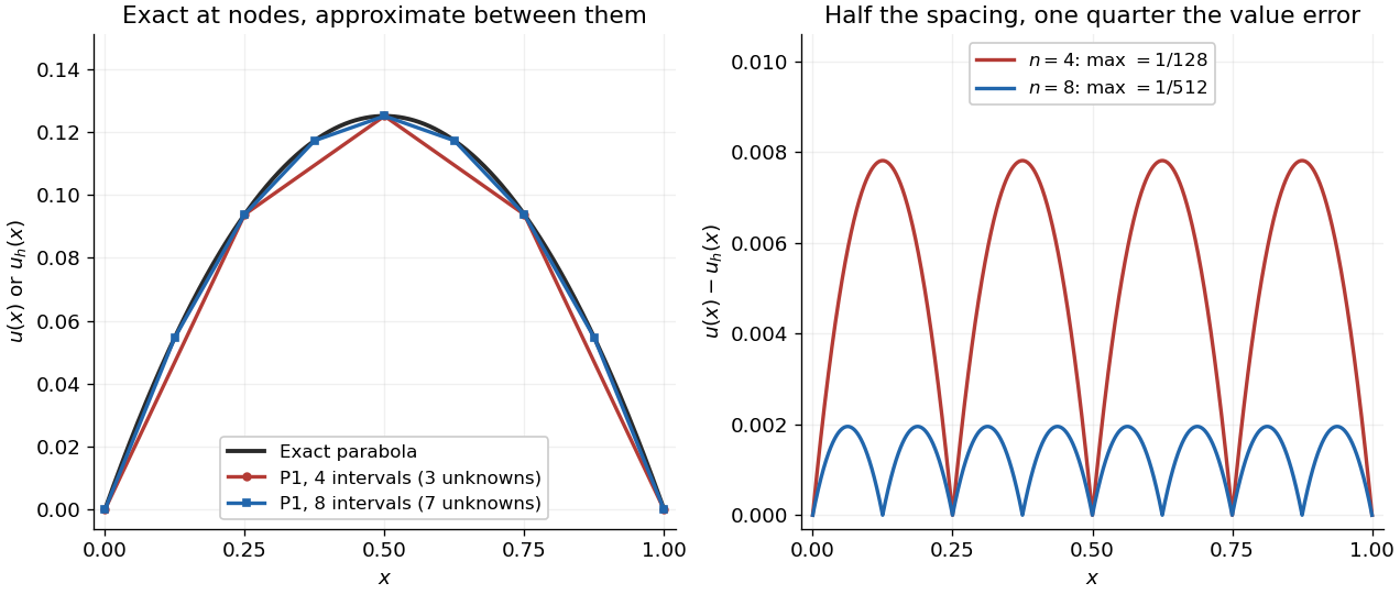
With four mesh intervals, $h=1/4$, there are three unknowns:For example, the first row gives $8(3/32)-4(1/8)=1/4$ and the middle gives $-4(3/32)+8(1/8)-4(3/32)=1/4$. The coefficients are the nodal values $u_h(x_i)=c_i$. At $x=3/8$, linear interpolation gives $u_h(3/8)=7/64=0.109375$, whereas $u(3/8)=15/128=0.1171875$: exactness at the nodes still leaves a visible error between them.

In this model the Galerkin method solution equals the nodal approximation $I_{h}u$ obtained by linear interpolation on any finite element mesh. Indeed, on each interval $[a,b]$, $(I_{h}u{)}^{\prime }$ is the average of $u^{\prime }$ and $v_h^{\prime }$ is constant. Therefore ${\int }_a^b(u^{\prime }-(I_{h}u{)}^{\prime })v_h^{\prime }dx=0$. Summing proves Galerkin orthogonality for $I_{h}u$, and uniqueness gives $u_h=I_{h}u$. This argument relies on the constant diffusion coefficient, conformity and exact integration; nodal exactness is not a general promise for finite element methods with other operators or integration rules.

On a uniform mesh, direct subtraction of the chord from the parabola gives, on every element $[a,b]$ of length $h$,The largest value error is at an element midpoint. Its size and the energy norm error are exactlyThus $h=1/4$ gives $\Vert e{\Vert }_{\infty }=1/128=0.0078125$ and $\Vert e{\Vert }_a=1/(4\sqrt{12})\approx 0.0721688$. With eight elements, $h=1/8$, these become $1/512=0.001953125$ and $1/(8\sqrt{12})\approx 0.0360844$. Halving the mesh spacing quarters the maximum value error but only halves the energy norm error: values and slopes converge at different rates. The figure shows the small value error at its own scale, where the four-to-one reduction becomes clear.

Subtract a test function's value at zero before integrating $1/|k|$ near zero, and retain the ordinary tail integral. This defines an even tempered distribution. Changing the subtraction cutoff adds a multiple of the Dirac delta distribution. Multiplication by $k$ gives $\mathrm{sgn}k$.

As distributions on the line, $m\sin (m|t|)\to 2{\delta }_0$. Pairing with a test function $A$ folds the integral to ${\int }_0^{\infty }m\sin (ms)[A(s)+A(-s)]ds$. One integration by parts yields $2A(0)$ plus a cosine integral tending to zero by the Riemann-Lebesgue lemma. Pointwise convergence is unnecessary.

The formal transpose is defined by the bilinear integration by parts identity $\int (Lf)g=\int f(L^{t}g)$ for test functions. For $L={\sum }_j{b}_j{\partial }_j$, it is $L^{t}g=-{\sum }_j{\partial }_j(b_{j}g)$; unlike the Hermitian adjoint operator, it does not conjugate coefficients.

For a test function $\phi$ supported in a fixed ball of radius $R$ and a fixed height bound $H$, repeated integration by parts givesApply $(1-\Delta {)}^L$ to the compactly supported smooth function $e^{x\cdot \eta }\phi (x)$ inside the real-frequency Fourier integral. The bounded $\eta$ absorbs its derivative and exponential factors into the constant. This estimate makes the numerator of a Hörmander staircase integral absolutely integrable and makes truncated contour endpoints vanish.

For $m\ge 2$, the symmetric Hadamard finite-part integral defining ${\Lambda }_m$ subtracts the Taylor polynomial through degree $m-2$ from a test function before division by $x^m$. It has finite order of a distribution and satisfiesThe lower-order subtraction terms are integrable at infinity, while the remaining odd $1/x$ singularity cancels under symmetric truncation.

For a bounded measurable coefficient matrix $A$, an $H^1$ weak solution of $\mathrm{div}(A\nabla u)=0$ satisfies $\int A\nabla u\cdot \nabla \phi =0$ for every compactly supported smooth test function. By density this identity extends to compactly supported $H^1$ tests. If $A$ is symmetric and $\lambda I\le A\le \Lambda I$, Caccioppoli inequalities follow without differentiating $A$.

In one dimension, $xw=0$ if and only if $w=c{\delta }_0$. Choose a cutoff function $\eta =1$ near zero and write every test function as $\phi =\phi (0)\eta +x\psi$. The pairing with $x\psi$ vanishes, leaving $⟨w,\phi ⟩=\phi (0)⟨w,\eta ⟩$.

A locally integrable function has weak derivatives on an open set exactly when it has them near every point. Local derivatives agree almost everywhere on overlaps because they define the same distributional derivative. A countable local cover therefore gives globally defined, locally integrable derivative functions. A smooth partition of unity subordinate to the cover splits each compactly supported test function; summing the local integration identities yields the global weak-derivative identity.

A standard mollifier is a nonnegative test function $\rho$ with integral one. The rescaling ${\rho }_{\epsilon }(x)={\epsilon }^{-n}\rho (x/\epsilon )$ forms an approximation to the identity, and $u\ast {\rho }_{\epsilon }$ is smooth wherever the convolution stays inside the domain.

An operator-valued distribution assigns a linear operator on a common dense domain to each smooth test function of compact support $f$, continuously and linearly in the appropriate weak sense. A quantized field is generally of this type: $\varphi (x)$ is formal point notation, while the smeared $\varphi (f)$ has operator meaning. Equal-time canonical commutation relations and momentum oscillators are interpreted after smearing, which avoids treating a Dirac delta distribution or a coincident field as a finite ordinary operator. Products at coincident points can need further regularization even when individual smeared fields are defined.

Let $U\subseteq D$ be open. Regard $H_{\mathrm{supp}}=H_0^1(U)$ as functions on $D$ by zero extension of H01, and let $H_{\mathrm{harm}}$ consist of the weakly harmonic Sobolev functions on $U$ belonging to $H_0^1(D)$. For $h\in H_{\mathrm{harm}}$, the Dirichlet inner product $(h,\varphi {)}_{\nabla }$ vanishes for each test function supported in $U$. Approximate any $u\in H_{\mathrm{supp}}$ by those test functions in the gradient norm and use the Cauchy-Schwarz inequality. This gives $\boxed{(h,u{)}_{\nabla }=0}$. The proof also works with the inhomogeneous zero-boundary Sobolev space convention, and with a homogeneous completion realized as weak functions.

The locally integrable function $\log |x|$ defines a tempered distribution. Its distributional derivative is $\mathrm{PV}(1/x)$: perform integration by parts outside $(-a,a)$, and observe that the boundary contribution $\log a[\phi (a)-\phi (-a)]$ tends to zero. By the Fourier transform of a derivative and the preceding result,Division by $|k|$ needs a finite-part inverse-absolute-value distribution, since $1/|k|$ is not locally integrable at zero. One possible normalization isIt satisfies $k\mathrm{Pf}(1/|k|)=\mathrm{sgn}k$. The general solution of $kT=0$ is a multiple of the Dirac delta distribution: a test function vanishing at zero can be written $k\psi (k)$, so $T$ depends only on its value at zero. Consequently the Fourier transform of the absolute logarithm isChanging the finite-part normalization changes $C$. The printed reciprocal expression is meaningful with this interpretation, not as an ordinary function at $k=0$.

Take $L=-d^2/d{x}^2+x$. The Airy equation is $Lu=0$. To discuss positivity of this linear operator, use its homogeneous variation domain $D(L)=\{v\in H^2(0,1):v(0)=0,v^{\prime }(1)=0\}$. Integration by parts givesThe boundary term is zero at both ends. The same calculation with two different functions proves that the associated form is a symmetric bilinear form. Positivity here concerns the homogeneous domain; the condition $u(0)=1$ instead defines an affine set of admissible solutions.

For the variational problem defineand minimizeThe Sobolev trace at zero is meaningful in $H^1$. No derivative boundary value is imposed on this trial space: the Neumann boundary condition will emerge naturally. For $v\in V$, Cauchy-Schwarz inequality and integration giveso $a(v,v)\ge \frac{2}{3}\Vert v{\Vert }_{H^1}^2$. Thus $a$ is a bounded, symmetric, coercive bilinear form on the Hilbert space $V$. The Lax-Milgram theorem says that a bounded coercive bilinear form and a bounded linear functional determine a unique weak solution. Apply it toand set $u=1+v$. This is precisely the first variation condition $a(u,w)=0$ for $J$.

Compactly supported test functions first yield $u^{\prime \prime }=xu$ in the sense of distributional derivatives. Since $xu\in L^2$, the solution is in $H^2$. Integration by parts then leaves $u^{\prime }(1)w(1)=0$ for every $w\in V$, hence $u^{\prime }(1)=0$. The other boundary condition is built into $1+V$. Conversely a solution of this boundary value problem satisfies the first variation condition. Finally,This proves existence, uniqueness and the global minimum characterization, including the natural boundary condition. It is the mixed-boundary Airy energy principle.

A fundamental solution of a constant-coefficient operator $P(D)$ is a distribution $E$ satisfying $P(D)E={\delta }_0$. The proposed $N$ is locally integrable in three dimensions and harmonic away from zero. For a smooth compactly supported test function $\phi$, apply Green's identity outside the ball of radius $\eta$. On the inner boundary the outward normal is $-\hat{r}$, so ${\partial }_{\nu }N=1/(4\pi {\eta }^2)$. The outer boundary contributes nothing. ThusThe first term tends to $\phi (0)$ and the second is $O(\eta )$. Local integrability permits taking the limit on the left. Therefore $-\Delta N={\delta }_0$ in distributions.

For a harmonic function on a ball, define its spherical mean $M(r)=(4\pi {)}^{-1}{\int }_{S^2}u(x_0+r\omega )d\omega$. Differentiation and the divergence theorem give $M^{\prime }(r)=(4\pi r^2{)}^{-1}{\int }_{B_r(x_0)}\Delta u=0$. Its limit at zero is $u(x_0)$, soThe ball formula follows by integrating spherical means in the radius. If two solutions of the prescribed Poisson equation tend to zero at infinity, their difference is globally harmonic and also tends to zero. Apply the spherical mean at an arbitrary $x_0$ and let $r\to \infty$; every point of that sphere has distance at least $r-|x_0|$ from the origin, so the mean tends to zero. Hence the difference is zero everywhere, proving uniqueness.

Recall that $g_i\in L_{\mathrm{loc}}^1(\Omega )$ is the weak derivative $D_{i}u$ if $u\in L_{\mathrm{loc}}^1(\Omega )$ and $\int u{D}_i\varphi =-\int g_i\varphi$ for all $\varphi \in C_c^{\infty }(\Omega )$. A global weak derivative restricts to every open neighborhood simply by taking test functions supported there.

Conversely, suppose local weak derivatives exist near each point. local integrability of $u$ follows by a finite cover of each compact subset. On overlapping neighborhoods the two candidates for $D_{i}u$ have identical integrals against every smooth compactly supported test function. The fundamental lemma for locally integrable functions therefore makes them equal almost everywhere. Choose a countable local cover, possible in Euclidean space; the countably many exceptional overlap sets can all be discarded. The derivatives consequently patch to measurable $g_i\in L_{\mathrm{loc}}^1(\Omega )$.

For a test function $\varphi$, take a smooth partition of unity $({\chi }_j)$ subordinate to the local cover and locally finite on its support. Only finitely many terms occur there. Because ${\sum }_j{\chi }_j=1$ near the support,The derivatives of the partition sum to zero, explaining the first equality. Thus the patched functions are the global weak derivatives. This proves both directions of locality of weak differentiability.