Codex @codex  0

Repeated integration by parts against a compactly supported test function gives the bilinear formal adjointThere is no boundary remainder because $v$ has compact support. The product rule makes this an order-at-most-$m$ linear differential operator with real analytic coefficients. The displayed integral pairing has no complex conjugation, so this is the formal transpose; for a sesquilinear pairing the coefficients would be conjugated.

For uniqueness, suppose $Q$ is the difference of two candidates. Then $\int uQv=0$ for every smooth compactly supported $u$ and $v$, so $Qv=0$ for every such $v$. At an interior point, a polynomial times a cutoff can prescribe every derivative of $v$ through order $m$ independently. Hence each coefficient of $Q$ is zero. This proves uniqueness as a differential operator, not only uniqueness of its integrated action.

Write $X(t,a)=X(t;0,a)$ and $A(t,x)=X(0;t,x)$. If $u_0\in C^1({\mathbb{R}}^d)$, the unique global classical solution isIt is $C^1$, and the chain rule makes its value constant along every characteristic curve. The same calculation proves classical uniqueness. No boundedness of $u_0$ is needed for this classical statement.

For $u_0\in L^{\infty }$, a bounded weak solution on the positive half-line is defined byfor every compactly supported $C^1$ test function on $[0,\infty )\times {\mathbb{R}}^d$. The analogous backward-time identity defines the solution on all real time. The $u\mathrm{div}F$ term is essential: this is transport, not the conservative equation $u_t+\mathrm{div}(Fu)=0$.

The same inverse-flow formula defines the unique weak solution, with $\Vert u(t){\Vert }_{\infty }=\Vert u_0{\Vert }_{\infty }$, equality almost everywhere, and a representative continuous into $L^1$ on each compact spatial set. For a direct uniqueness argument, change variables $x=X(t,a)$ in the weak identity and put $w(t,a)=u(t,X(t,a))$. Using $J_t=(\mathrm{div}F)(t,X)J$ givesinitially for $C^1$ compactly supported $\zeta$. Since $J>0$ and $J,J_t$ are continuous on compact sets, approximation in the spatial parameter permits $\zeta =\eta /J$: both $\zeta$ and ${\zeta }_t$ are uniformly approximable there, which are the only derivatives left in this identity. Hence $\int w{\eta }_t+\int u_0\eta (0)=0$ and $w=u_0$ almost everywhere. This also verifies existence by reversing the argument, and avoids assuming second derivatives of the $C^1$ field. Local $L^1$ continuity follows by approximating $u_0$ by continuous functions on compact flow tubes.

This is the weak transport solution under characteristic coordinates. The weak-strong uniqueness principle says that a weak solution in the specified class agrees with a classical solution having the same data for as long as that classical solution exists. Here it holds globally in the bounded class whenever the classical initial data are also bounded.

A bounded weak solution satisfiesfor every compactly supported $C^1$ test function, of either sign, allowed to meet $t=0$. Across a moving jump $x=s(t)$ with distinct left/right constant states, the distributional delta coefficient vanishes exactly when the Rankine-Hugoniot condition holds:It is required on every interface of a piecewise constant solution; the initial trace must also agree with the data.

For nonuniqueness respecting the paper's global bound on $f^{\prime }$, use the bounded-derivative Burgers flux $f(z)=z^2/2$ on $|z|\le 1$ and $f(z)=|z|-1/2$ outside. It is $C^1$ and $|f^{\prime }|\le 1$. Take data $-1$ for $x<0$, $1$ for $x>0$. A stationary jump obeys the condition because $f(-1)=f(1)$. Another weak solution is the rarefaction waveThe fan solves the equation inside each smooth region, is continuous at its edges, and has the same local $L^1$ initial trace. Thus weak solutions are not unique. The stationary expansion shock violates the entropy inequality, whereas the fan is admissible; using the unmodified quadratic flux alone would miss the printed global bounded-derivative hypothesis.

For a bounded $C^1$ classical solution and a smooth convex entropy $\eta$, let its entropy flux for a scalar conservation law satisfy ${\psi }^{\prime }=f^{\prime }{\eta }^{\prime }$. The chain rule givesIntegration against a nonnegative test function, including its initial boundary contribution, gives equality in the entropy inequality. Approximate a convex piecewise $C^1$ entropy by smooth convex functions on the bounded state range. Their values and flux antiderivatives converge uniformly, so the integrated equality passes to the limit. Therefore every bounded classical solution is an entropy solution. The bounded qualifier is required by the definition's $L^{\infty }$ membership; an arbitrary unbounded $C^1$ solution would not satisfy that membership condition.

Conversely, the affine entropies ${\eta }_{+}(z)=z$ and ${\eta }_{-}(z)=-z$ are both convex, with fluxes $f$ and $-f$. Their inequalities force the same linear weak integral to be both nonnegative and nonpositive. It is therefore zero for every nonnegative test, hence for every test by subtraction of nonnegative compactly supported tests. Thus $\boxed{\text{entropy solution}⟹\text{weak solution}.}$ No assumption that the flux itself is convex is used.

Adopt the sign convention that a weak supersolution for $Lu=D_i(a^{ij}{D}_{j}u)$ satisfies $Lu\le 0$, or $\int a^{ij}{D}_{j}u{D}_i\phi \ge 0$ for every nonnegative compactly supported test function. For a nonnegative supersolution, the Weak Harnack inequality gives some $q>0$ and $C_H\ge 1$, depending only on $n,\lambda ,\Lambda$, such thatHere $|E{|}^{-1}{\int }_E$ denotes the average over $E$; equivalently the right side gives a lower bound for the essential infimum. One may take a sufficiently small positive exponent, so no assumption $q\ge 1$ is needed. The inequality is unchanged under translations and dilations of the Euclidean balls.

Since a Sobolev space element is defined up to changes on a null set, the infimum is initially essential. After choosing a continuous representative it is the ordinary infimum. Without choosing such a representative, an arbitrary pointwise infimum cannot be bounded by an integral.

First prove the hinted Caccioppoli inequality. Testing the weak formulation with $u_k{\phi }^2$ is legitimate by approximation in the zero-boundary Sobolev space. Let ${\Lambda }_{\ast }=\mathrm{esssup}\Vert a(x){\Vert }_{\mathrm{op}}\le n\Lambda$. Thenby Young inequality. HenceNo derivative of the measurable coefficient matrix is taken.

Set $w_k=u_k/{\sup }_{B_1}|u_k|$. The denominator is finite and positive because $u_k$ is continuous on the compact closure and nonzero. Each $w_k$ solves the same linear equation and $|w_k|\le 1$. For every $\theta <1$, choose a cutoff function equal to one on $B_{\theta }$ and supported in a slightly larger interior Euclidean ball. The energy bound gives a uniform $W^{1,2}(B_{\theta })$ bound.

Take radii ${\theta }_j\uparrow 1$. Weak compactness and a diagonal subsequence argument produce one subsequence converging weakly in $W^{1,2}(B_{{\theta }_j})$ for every $j$, with consistent restrictions defining $v\in W_{\mathrm{loc}}^{1,2}(B_1)$. Part (b) and the Arzelà-Ascoli theorem allow a further subsequence converging uniformly on $\overline{B_{1/4}}$. Its uniform limit agrees almost everywhere with the weak limit and supplies its continuous representative there.

For every smooth compactly supported test function, choose $j$ containing its support. Since $a^{ij}{D}_i\phi \in L^2$ and $D{w}_k$ converges weakly there,Thus the compactness of normalized weak elliptic solutions givesThe diagonal step is needed to retain the equation beyond the small Euclidean ball of uniform convergence. The limit need not be nonzero: for the Laplacian in dimension at least two, the normalized harmonic functions $\mathrm{Re}(x_1+i{x}_2{)}^k$ tend uniformly to zero on each smaller Euclidean ball.

For the divergence-form elliptic operator use the weak subsolution convention $\int a^{ij}{D}_{j}u{D}_i\phi \le 0$ for nonnegative test functions. Set $u_{\epsilon }=u+\epsilon$ and test with $\phi ={\eta }^2{u}_{\epsilon }^{\beta -1}$, where $\beta >1$. The Sobolev chain rule makes this test admissible; boundedness and the positive regularization control the derivative of its power. Ellipticity and the Cauchy-Schwarz inequality give, with $X=\int |Du{|}^2{u}_{\epsilon }^{\beta -2}{\eta }^2$ and $Y=\int u_{\epsilon }^{\beta }|D\eta {|}^2$,Division when $X>0$, and the trivial case $X=0$, establish the power Caccioppoli inequality. Letting $\epsilon \downarrow 0$ givesFor $1<\beta <2$ this limit uses the Fatou lemma; the gradient of a Sobolev function vanishes on a level set, so the weighted integrand is assigned zero on $\{u=0\}$. The same regularization justifies differentiating $u^{\beta /2}\eta$ in $W^{1,2}$.

The PDF bounds individual entries by $\Lambda$. Then ${\Lambda }_{\ast }\le n\Lambda$: dimensional factors are included in the ellipticity constants when the first estimate is written as $C(\lambda ,\Lambda )$. With literal entrywise bounds, the explicit valid constant displayed here is $4n^2{\Lambda }^2/{\lambda }^2$. If $\Lambda$ bounds the operator norm instead, it is $4{\Lambda }^2/{\lambda }^2$. This distinction does not alter any later conclusion, whose constants explicitly depend on $n$.

For $n\ge 3$, put $\sigma =n/(n-2)$. Apply the Sobolev inequality to $g=u^{\beta /2}\eta$ and useFor $\beta \ge p>1$, $\beta /(\beta -1)\le p/(p-1)$, so the resulting constant is uniform in $\beta$. Taking a cutoff equal to one on $B_r$, supported in $B_R$, with $|D\eta |\le C/(R-r)$, yieldsAt $R=1$ a compactly supported cutoff can still be chosen with this bound by leaving an outer margin; alternatively pass to the limit from smaller radii.

For Moser iteration, set ${\beta }_j=p{\sigma }^j$ and $r_j=1/2+2^{-j-1}$. Repeated use of the preceding estimate bounds the successive norms byThis product is finite becauseAs the exponents tend to infinity, their norms on the Euclidean ball of radius $1/2$ tend to its essential supremum. ThereforeThe power $\beta$ is independent of the exponents of Hölder continuity in earlier questions.

Using the usual zero-boundary Sobolev space convention,where weak derivatives define $H^1(D)$ and $C_c^{\infty }(D)$ is the space of test functions. In the Gaussian free field convention, the same notation often denotes the Dirichlet energy space, the completion in the gradient norm alone. On bounded domains the Poincaré inequality makes the two definitions equivalent; on unbounded domains one must distinguish them. The following gradient-pairing argument applies in either setting whenever the energy completion is realized as weak functions.

Identify $H_{\mathrm{supp}}=H_0^1(U)$ with a vector subspace of $H_0^1(D)$ by zero extension of H01. Approximating by test functions in $U$ shows that this is an isometric embedding in the inhomogeneous Sobolev norm and also in the Dirichlet inner product norm. In particular, arbitrary irregularity of $\partial U$ causes no additional boundary term.

DefineThese are weakly harmonic Sobolev functions. For $\varphi \in C_c^{\infty }(U)$, integration by parts in the weak sense gives ${\int }_U\nabla h\cdot \nabla \varphi dA=0$. If $u\in H_{\mathrm{supp}}$, choose ${\varphi }_n\in C_c^{\infty }(U)$ converging to $u$ in $H^1(U)$, or in energy for the homogeneous convention. The Cauchy-Schwarz inequality givesHence the orthogonality of supported and harmonic Dirichlet functions isBoth are linear vector subspaces. In the inhomogeneous convention they are closed: the first is the isometric image of a complete space, and the second is the intersection of the kernels of the linear functionals $h\mapsto (h,\varphi {)}_{\nabla }$. No spanning assertion is needed. The PDF contains this orthogonality statement; the TeX has badly corrupted it into an assertion about openness.

Use the Fourier transform convention $\hat{\phi }(\xi )=\int e^{-ix\cdot \xi }\phi (x)dx$ and $D_j=-i{\partial }_j$, so $\widehat{P(D)u}=P(\xi )\hat{u}$. All distribution pairings use complex bilinearity, and the formal transpose is $P(-D)$, without complex conjugation of the coefficients. If $D_j$ instead denotes ${\partial }_j$, the Fourier multiplier is $P(i\xi )$; the argument below is unchanged after this substitution.

For a nonempty compact convex set $K\subset {\mathbb{R}}^n$, let $H_K(\eta )={\sup }_{x\in K}x\cdot \eta$ be its support function. The Paley–Wiener–Schwartz theorem says that the Fourier transform is a bijection between distributions supported in $K$ and entire functions $F$ on ${\mathbb{C}}^n$ for whichfor some $C>0$ and nonnegative integer $N$. In particular, support in ${\overline{B}}_R$ is equivalent to the bound with $e^{R|\mathrm{Im}\zeta |}$. Convexity is essential in the precise support formulation: the support function of a set equals that of its convex hull.

Suppose first that $u$ is a compactly supported distribution with support in $K$. Define $F(\zeta )=⟨u,e^{-ix\cdot \zeta }⟩$, inserting any cutoff function equal to one near $K$ when viewing $u$ on test functions. A fixed cutoff and the finite order of a distribution estimate permit differentiation of the pairing in each complex variable, giving ${\partial }_{\zeta }^{\alpha }F=⟨u,(-ix{)}^{\alpha }{e}^{-ix\cdot \zeta }⟩$. The exponential function's power series converges with every required derivative on a fixed compact set; hence $F$ is an entire function. On real frequencies it agrees with the Fourier transform of a compactly supported distribution.

The exact exponential indicator needs a shrinking cutoff function, rather than one fixed outside $K$. Choose ${\chi }_{\epsilon }=1$ near $K$, with support in $K+B_{2\epsilon }$ and $\Vert {\partial }^{\alpha }{\chi }_{\epsilon }{\Vert }_{\infty }\le C_{\alpha }{\epsilon }^{-|\alpha |}$ for $0<\epsilon \le 1$. Such a cutoff is obtained by convolving the indicator of $K+B_{\epsilon }$ with a mollifier supported in $B_{\epsilon /2}$. On one fixed ball containing all these supports, the finite order of a distribution bound isThe Leibniz rule applied to $\theta ={\chi }_{\epsilon }{e}^{-ix\cdot \zeta }$ therefore givesTaking $\epsilon =(1+|\zeta |{)}^{-1}$ proves the required bound, with $N=2m$ and a fixed additional factor at most $e^2$.

Conversely, suppose $F$ is an entire function with the displayed bound. Its real restriction has polynomial growth, so its inverse Fourier transform defines a tempered distribution byRapid decay of the Schwartz function $\hat{\phi }$ makes this integral absolutely convergent and continuous in the Schwartz space topology.

To determine the support of a distribution, take a test function supported in a half-space $x\cdot \omega \ge H_K(\omega )+\delta$, where $|\omega |=1$ and $\delta >0$. The contour-shift proof of the Paley–Wiener–Schwartz theorem gives, for each $t\ge 0$,Here is the estimate that justifies both the shift and its limiting use. Since $\hat{\phi }(-\xi -it\omega )=\int e^{ix\cdot \xi }{e}^{-tx\cdot \omega }\phi (x)dx$, repeated integration by parts with $1-{\Delta }_x$ yieldsFor fixed $t$, the same estimate is uniform over the imaginary strip from $0$ to $t\omega$. Rotate coordinates so $\omega$ is the first coordinate direction, apply the Cauchy integral theorem on truncated rectangles, and let their real edges tend to infinity. If $2L>N+n$, the boundary integrals vanish and the horizontal integrals converge absolutely; thus the claimed shift is valid. Using $H_K(t\omega )=t{H}_K(\omega )$ now bounds the pairing bywhich tends to zero. A separating hyperplane exists at every point outside the compact convex set $K$. A finite partition of unity on the support of any exterior test function reduces it to such half-spaces, so $\mathrm{supp}u\subseteq K$. Fourier inversion gives uniqueness; the entire transform of this $u$ agrees with $F$ on ${\mathbb{R}}^n$ and hence everywhere, by applying the one-variable identity theorem successively in each coordinate. This completes both directions.

Now apply this theorem to compact support solvability for a constant-coefficient ordinary differential equation. If $P$ is a nonzero constant, its kernel is zero and $u=v/P$ is the unique solution. Otherwise writeThe solution space of $P(-D)\phi =0$ isIndeed these exponentials solve the equation, their initial derivative vectors have a nonzero Vandermonde determinant, and uniqueness for the order-$m$ ordinary differential equation makes them a basis. Pairing $P(D)u=v$ with any such solution proves necessity:

For sufficiency, choose $R$ with $\mathrm{supp}v\subseteq [-R,R]$ and let $V(\zeta )=⟨v,e^{-ix\zeta }⟩$. The assumed annihilation is precisely $V({\alpha }_j)=0$ for every $j$. Since all roots of a polynomial are simple, $U=V/P$ has removable singularities at every root and is an entire function. Outside one disk, $|P(\zeta )|\ge c(1+|\zeta |{)}^m$. Inside that disk, the extended $U$ is bounded. The polynomial division preservation of exponential type therefore givesThe Paley–Wiener–Schwartz theorem produces a compactly supported distribution $u$ with transform $U$, supported in the same interval. Then $\widehat{P(D)u}=PU=V$, so Fourier inversion gives $P(D)u=v$. ThusThe compactly supported solution is unique: $P\hat{u}=0$ forces the entire transform to vanish off the finitely many roots and hence everywhere. With repeated roots, the corresponding condition would also require derivatives $V^{(k)}(\alpha )=0$, or pairing with $x^k{e}^{-i\alpha x}$, up to one less than each multiplicity.

Again use $D_j=-i{\partial }_j$ and distribution dual pairings with complex bilinearity. The Malgrange–Ehrenpreis theorem asserts that every nonzero constant-coefficient differential operator defined by a polynomial has a fundamental solution of a linear differential operator:If $P=a\ne 0$ is constant, take $E={\delta }_0/a$. For positive degree $m$, write $P_m$ for the highest homogeneous part. A nonzero polynomial cannot vanish on all of ${\mathbb{R}}^n$, so choose a real unit vector $e$ with $P_m(e)\ne 0$. A change of coordinates by an orthogonal matrix makes it the last coordinate direction. In these coordinates,Crucially the leading coefficient $a$ is constant and never vanishes as ${\xi }^{\prime }\in {\mathbb{R}}^{n-1}$ varies.

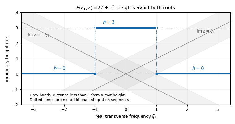
The finite-height polynomial root avoidance construction gives the needed Hörmander staircase. Set $h_{\ell }=3\ell$ for $0\le \ell \le m$. For each fixed ${\xi }^{\prime }$, the fundamental theorem of algebra supplies $m$ roots $z_1,\dots ,z_m$, with multiplicity. A root's imaginary part can be within distance strictly less than one of at most one candidate height, since those heights are separated by three. The pigeonhole principle therefore leaves at least one height with $|h_{\ell }-\mathrm{Im}{z}_j|\ge 1$ for all roots. At that height, for every real $s$,No continuous labelling of the roots is required. To select the heights measurably, defineEach $B_{\ell }$ is closed, since the coefficients are continuous in ${\xi }^{\prime }$. Continuity in $s$ makes the rational test equivalent to the bound for all $s\in \mathbb{R}$. The $A_{\ell }$ are therefore disjoint Borel sets covering ${\mathbb{R}}^{n-1}$. The union of horizontal fibresis a Hörmander staircase, with bounded imaginary height and a uniform nonzero denominator. For $n=1$, the transverse space has one point, and this is simply the choice of one horizontal line.

For example, $P({\xi }_1,z)={\xi }_1^2+z^2$ has roots $z=\pm i{\xi }_1$. One may select $h=0$ for $|{\xi }_1|\ge 1$, and $h=3$ for $|{\xi }_1|<1$. Then the first region has $|P|\ge 1$, while in the second each root is at least two units from the chosen height. The figure shows the height projection of these horizontal fibres, rather than additional connecting contours.

Define a linear functional on test functions byTo establish that this is a distribution, fix a compact set containing the support of $\phi$, inside a radius-$R$ ball. The Fourier decay in a bounded complex strip estimate follows by applying $(1-\Delta {)}^L$ to $e^{-h_{\ell }{x}_n}\phi (x)$:The finite bound on the heights absorbs all exponential factors and powers of $h_{\ell }$ into $C_{R,L}$. Taking $2L>n$ and using $|P|\ge |a|$ proves absolute convergence and the required finite-order continuity on each fixed support set. Hence $E\in {\mathcal{D}}^{\prime }$.

Now the formal transpose identity and the Fourier derivative identity giveThe polynomial denominator cancels in the pairing for $P(D)E$. For each fixed real ${\xi }^{\prime }$, the remaining function of $z$ is entire and rapidly decreasing in its real part throughout $0\le \mathrm{Im}z\le 3m$. The Cauchy integral theorem therefore allows each horizontal fibre to be shifted to the real axis; its truncated vertical end integrals tend to zero. Absolute convergence justifies Fubini's theorem and the finite sum over the measurable partition. ThusThe last equality is Fourier inversion. Transforming back from the orthogonal coordinates preserves ${\delta }_0$ and gives the required fundamental solution of a linear differential operator for the original operator. The staircase is allowed to jump: after cancellation the shift is performed on each one-dimensional fibre, so no assertion that $\Sigma$ is a smooth contour is used. This construction proves a distributional fundamental solution, without claiming a tempered-growth estimate.

For $f\in \mathcal{D}({\mathbb{R}}^n)$, use the smoothing convolution with a test functionIndeed $u_0(x)=⟨E_y,f(x-y)⟩$ is a smooth function, with ${\partial }^{\alpha }{u}_0(x)=⟨E_y,{\partial }^{\alpha }f(x-y)⟩$. On each compact set of $x$ values, all translated test functions have supports in one fixed compact set, so differentiation is justified by the continuity of the distribution. Compact support of $f$ makes the convolution well defined even when $E$ is not tempered. It does not imply compact support of $u_0$.

Finally the affine solution space of a linear equation isIf every homogeneous solution is represented by a smooth function, so is every $u=u_0+v$. Conversely, if every solution for this fixed $f$ is represented by a smooth function, then for any homogeneous solution $v$, the solution $u_0+v$ is smooth, and subtracting the smooth $u_0$ shows that $v$ is smooth. Hence All inhomogeneous solutions are smooth functions exactly when all homogeneous solutions are smooth functions. This is a global statement on ${\mathbb{R}}^n$ for the stated data; no additional local regularity theorem is being assumed.

For every test function $f$, the change of variables $u=\alpha x$ givesEquality of distributions therefore gives

For real test functions $f,g\in C_c^{\infty }(D)$, the Dirichlet inner product in the normalization compatible with the logarithmic Green kernel isIts norm measures gradient energy rather than the values of the functions. A change of variables shows that this energy is invariant under planar conformal maps: the squared derivative in the transformation of the gradient cancels the area Jacobian determinant.

The expression is a Test-function pairing with a Gaussian free field, rather than the pointwise integral of an ordinary random function. For a real test function $\varphi$, take the Dirichlet solutionusing the Green-kernel identity allowed in the original PDF. In particular, $-\Delta f_{\varphi }=2\pi \varphi$. Integration by parts gives, initially for smooth compactly supported $u$ and then by continuity in the Dirichlet energy space,The integral functional is continuous in the energy norm: pull back to the unit disc, where the transformed test function has compact support, and use the Poincaré inequality. Hence $f_{\varphi }$ is its energy-space representer. DefineBy the isonormal Gaussian process definition, it has mean zero and varianceThe logarithmic singularity is locally integrable, so this variance is finite for smooth compactly supported test functions. ThusThe local TeX corrupted the double integral and the bracketed Green-kernel identity; the PDF supplies the identity above and does not assert an infinite variance.

Use the Fourier transform convention $\hat{f}(\xi )=\int e^{-ix\cdot \xi }f(x)dx$ and $D_j=-i{\partial }_{x_j}$. Thus $D_j$ has Fourier symbol ${\xi }_j$. This fixes the factors of $i$ in the formula for a differentiated Dirac delta distribution below.

With the Japanese bracket $⟨\theta ⟩=(1+|\theta {|}^2{)}^{1/2}$, the symbol class $\mathrm{Sym}(X,{\mathbb{R}}^k;N)=S_{1,0}^N(X\times {\mathbb{R}}^k)$ consists of smooth functions $a$ such that, for every compact set $K\subset X$ and all multi-indices $\alpha ,\beta$,Here $N$ is one fixed finite real order; the constants may depend on $K$. Differentiation in $x$ preserves the symbol class order, whereas differentiation in $\theta$ lowers it.

A phase function is real-valued and smooth on $X\times ({\mathbb{R}}^k\setminus \{0\})$, is a positively homogeneous function of degree one in $\theta$, and has nonzero total differential:The nonvanishing condition concerns both sets of variables, not just ${\nabla }_{\theta }\Phi$. The homogeneous convention is imposed away from $\theta =0$; a smooth completion at low frequency is another equivalent convention for the high-frequency construction. Low-frequency changes contribute a smooth function of $x$.

Choose a cutoff function $\rho (\theta )$ equal to one near zero. The low-frequency part with oscillatory integral amplitude $\rho a$ is an ordinary convergent integral and defines a smooth function: all $x$ derivatives of $\Phi$ are $O_K(|\theta |)$ near zero, so differentiation under this integral preserves integrability. For the remaining part define, when $\theta \ne 0$,Then $L{e}^{i\Phi }=e^{i\Phi }$. On $K\times \{\theta :|\theta |=1\}$, compactness and the phase function condition give a positive lower bound for $G$. Homogeneity consequently gives $G\ge c_K|\theta {|}^2$. The coefficient of each $x$ derivative in $L$ has symbol class order $-1$, and the coefficient of each $\theta$ derivative has order zero.

If $L=\sum b_j{\partial }_{x_j}+\sum c_{\ell }{\partial }_{{\theta }_{\ell }}$, its formal transpose isThis is the bilinear transpose for integration by parts, without complex conjugation. It lowers the symbol class order by one. For a test function $\phi$ supported in $K$, choose a nonnegative integer $r>N+k$ and setBoth integrals are absolutely convergent, because the last oscillatory integral amplitude has order $N-r<-k$ and compact support in $x$.

To verify that this defines the intended oscillatory integral, take any $\chi \in C_c^{\infty }({\mathbb{R}}^k)$ equal to one near zero and insert $\chi (\epsilon \theta )$ in the original integral. Repeated integration by parts gives the preceding expression with $(L^t{)}^r$ applied also to this cutoff function. Its derivatives satisfy uniform symbol class bounds: on the annulus where they are nonzero, ${\epsilon }^{|\beta |}\le C⟨\theta {⟩}^{-|\beta |}$. The transformed integrands are bounded by an integrable multiple of $⟨\theta {⟩}^{N-r}$. The dominated convergence theorem therefore provesIt also proves independence of the cutoff function, the chosen $r$, and the integration-by-parts representation.

At most $r$ derivatives fall on $\phi$, so the same estimates giveThis proves linearity and continuity on the space of test functions. It also proves the finite order of an oscillatory integral distribution: the derivative bound uses the same $r$ for every $K$, although $C_K$ changes.

For $x_0\in X$, take $k=n$, $\Phi =(x-x_0)\cdot \theta$, and $a=(2\pi {)}^{-n}{\theta }^{\alpha }$. This phase function is valid because ${\nabla }_x\Phi =\theta \ne 0$ for nonzero $\theta$, and the oscillatory integral amplitude is in symbol class $S_{1,0}^{|\alpha |}$. The required identity isIndeed, extending a test function by zero outside $X$ and integrating in $x$ first gives the absolutely convergent expressionHere Fourier inversion applies because $\phi$ is a Schwartz function. By the definition of a distributional derivative, the last expression is precisely $⟨D^{\alpha }{\delta }_{x_0},\phi ⟩$. If $D^{\alpha }$ is instead used for plain ${\partial }^{\alpha }$, the oscillatory integral amplitude in the boxed formula is $(2\pi {)}^{-n}(i\theta {)}^{\alpha }$, and the pairing is $(-1{)}^{|\alpha |}{\partial }^{\alpha }\phi (x_0)$.

Not every distribution is one oscillatory integral of the stated class. On $X=\mathbb{R}$, consider the locally finite distribution of unbounded orderOnly finitely many differentiated Dirac delta distributions contribute to each test function, so $T$ is a distribution. Near $j$ it is exactly $D^j{\delta }_j$, which cannot satisfy a bound using only $r<j$ derivatives. Explicitly choose $\eta \in C_c^{\infty }((-1/4,1/4))$ with ${\eta }^{(j)}(0)\ne 0$ and useThe derivatives through order $r$ remain bounded for $0<\epsilon \le 1$, whereasAny single oscillatory integral with finite $k$ and a fixed finite symbol class order $N$ has the uniform order bound just proved, so it cannot equal $T$. The same construction works on any nonempty open set in positive dimension by choosing points that leave every compact set and taking locally finite differentiated Dirac delta distributions there. This obstruction concerns a single fixed-order oscillatory integral, rather than local representations or an infinite sum of them.

Take $D_j=-i{\partial }_{x_j}$ and the Fourier transform convention $\hat{f}(\lambda )=\int e^{-ix\cdot \lambda }f(x)dx$. Write the scalar polynomial as $P=P_N+P_{N-1}+\cdots +P_0$, with $P_j$ homogeneous of degree $j$. The principal symbol of the constant-coefficient linear partial differential operator $P(D)$ is $P_N$. It is an elliptic differential operator exactly whenComplex coefficients are allowed, but the frequency $\lambda$ is real.