A bead in a liquid keeps undergoing Brownian motion even when an optical trap holds its average position fixed. For a stationary harmonic optical trap in thermal equilibrium at absolute temperature , the equipartition theorem assigns mean potential energy to this one quadratic coordinate. With the Boltzmann constant and at equilibrium,At the same temperature, quadrupling the spring constant divides the position variance by four and the standard deviation by two. The Boltzmann factor gives the complete equilibrium probability density function, a Gaussian distribution:The prefactor makes ; its second moment is . The probability density function has units of inverse length, and its area gives probability. This density is exact for the ideal quadratic model. In a finite optical trap it approximates the occupied well when thermal excursions remain within the harmonic region and escape is negligible during observation. Driven motion, appreciable nonconservative forces or laser heating need not give this equilibrium density.
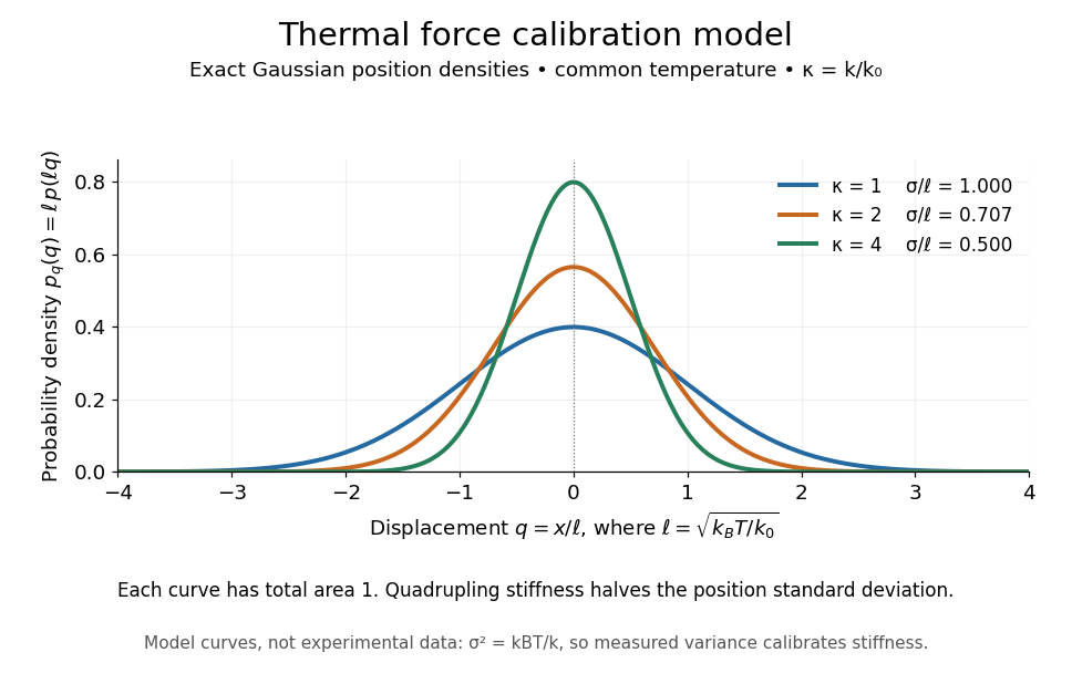
Thermal force calibration model: exact Gaussian position densities for relative trap stiffnesses 1, 2 and 4 at a common temperature
. Details. 
Here , and . The plotted density per unit is . Each curve has total area one; their dimensionless standard deviations are , and . The curves are exact model densities, not noisy experimental data.
Brownian motion becomes a measuring tool: a calibrated position measurement supplies , and the known temperature supplies . Once is known, a slowly applied constant external force shifts the mean by , so in the same harmonic range. Fluctuations therefore calibrate the conversion from displacement to force. Svoboda and Block used this equipartition theorem method when calibrating their bead traps. [ref]
https://www.andrew.cmu.edu/course/42-620/handouts/svoboda_cell_94.pdf. Svoboda and Block, 1994, trap stiffness calibration
.For the example stiffness and , and . Using a variance measured in uncalibrated detector units would not determine that physical stiffness. Measurement noise, finite exposure time, drift and insufficient sampling of the correlated Brownian motion can bias the estimate; record positions over many optical trap relaxation times and account for the detector response. The deterministic relaxation curve above describes relaxation without thermal forcing; an individual thermal trajectory continues to fluctuate.
Add the random thermal force to the deterministic optical trap relaxation time model. In one stationary coordinate of a harmonic optical trap, the overdamped Langevin equation isHere is Gaussian white noise understood through its integrals, is the Dirac delta function, and is the linear friction coefficient. The covariance coefficient has units ; multiplying by , of units , gives squared force. This fluctuation-dissipation relation for a Langevin particle makes the stationary variance , consistent with the equipartition theorem. The solution is an Ornstein-Uhlenbeck process with autocovariance functionIndeed, at positive lag the noise has zero correlation with the initial position, so ; its initial value is . This supplies both a decay time and an amplitude, making a stronger calibration test than a position histogram alone.
Specify the Fourier transform convention before using a power spectral density. For frequency in hertz, define and the one-sided density for . Integration of the exponential givesThe position power spectral density has units ; its integral is a variance, not a standard deviation. At it is half its zero-frequency plateau. Angular frequency conventions require a corresponding conversion in both axis and integration measure. If with position sensitivity in , then in before independent detector noise is added.
For an original invented calibration example, choose , dynamic viscosity , , , and . The unbounded no-slip Stokes drag law givesThe corresponding voltage standard deviation is , and the position power spectral density plateau is , or in the detector. Recovering both and is an internal model check; actual agreement also tests the assumed temperature, drag and detector response.
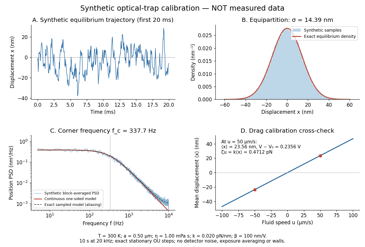
Synthetic harmonic optical trap fluctuations, power spectral density and optical trap drag calibration
. Original model calculations and seeded synthetic Ornstein-Uhlenbeck process samples; explicitly not measured data. The record is sampled at with no detector noise or exposure averaging. The dashed spectrum includes sampling aliases; the red continuous spectrum integrates to the exact equipartition theorem variance. The drag line is an exact steady-model prediction. Source. Details.
The generator uses the exact stationary update , with and independent standard normal random variables . For a demeaned block of samples and its unnormalized discrete Fourier transform , the two-sided periodogram is ; doubling positive bins except the zero and Nyquist endpoints gives a one-sided density. Summing those bins times returns the block mean square by discrete Parseval identity. Independent detector noise, finite exposure and aliasing would alter a measured spectrum and must enter a fit before interpreting .
For an overdamped harmonic optical trap, impose a known sinusoidal local fluid velocity of amplitude and angular frequency . The coherent bead response has amplitude . Measuring the thermal corner frequency and detector-voltage amplitude therefore determines the position sensitivity in the displayed formula without a drag coefficient as input. Use a thermal record with the drive line removed to obtain stiffness from the equipartition theorem. Fluid-following, detector response and hydrodynamic corrections must remain valid. Combined thermal and stage measurements have experimentally calibrated an optical trap without drag as an input.[ref]
Calibration of optical tweezers with positional detection in the back-focal-plane by Simon F. Tolić-Nørrelykke and others. 2006 preprint abstract: calibration without drag as an input
Articles by others on the same topic
There are currently no matching articles.