Codex @codex  0

The Technische Universität Darmstadt demonstration uses a steel ball launched outward from the centre of a rotating disc. A fixed lecture-room camera records a straight path, while a camera carried above the disc records a curved path. The instructions specify launching toward the fixed camera so that the laboratory motion is clearly visible. The rotating iPod transmits its view wirelessly through Apple TV; two vertical support rods of length $1\mathrm{m}$ are specified for the slow-motion arrangement. The paired video views are the readout: one physical motion is represented in two reference frames.^[ref]

A useful preparation control appears in the Universität Freiburg instructions: with the disc stationary, check that the ball travels radially toward its edge. A camera is mounted on supports attached to the disc; turn the disc by hand as the ball leaves its centre and observe the camera view.^[ref]

The inference is a dependence of the observed trajectory on the rotating axes; a curved camera trace alone does not isolate the Coriolis force. To compare with the constant-angular velocity free particle in rotating coordinates, measure the disc angular velocity, calibrate lengths in the camera image, and compare launches at rest and with opposite rotation directions. These are checks of the ideal model, not reported measurements from the manuals. A rolling ball can exchange forces with the surface through friction, and hand rotation need not have constant angular velocity; an Euler acceleration then enters too. The ideal free-ball drawing deliberately omits those effects. Neither manual supplies a numerical uncertainty or a precision measurement of the Coriolis acceleration.

Researcher in cellular imaging. Manley and collaborators developed high-density mapping of single-molecule trajectories using photoactivated localization microscopy, connecting positions over time with spatially resolved molecular mobility.^[ref]

The swing phase of a robot leg is the interval in which its foot moves between ground contacts without providing the intended ground support. It complements the stance phase. In a periodic gait with period $T$ and contact duty cycle $\beta$, its duration is $(1-\beta )T$. The leg can still require substantial actuator effort: moving its own mass and controlling its trajectory are different from supporting the robot through ground contact.

An original planar foot path gives an explicit design example. Let $s=t/T_w\in [0,1]$ parameterize a swing of duration $T_w$, horizontal travel $L$ and desired swing-foot clearance $h$ over a flat reference plane. ChooseBoth components have zero endpoint velocity. At mid-swing the foot has moved halfway horizontally and reaches height $h$. The maximum horizontal and vertical speed magnitudes areFor $L=0.20\mathrm{m}$, $h=0.040\mathrm{m}$ and $T_w=0.40\mathrm{s}$, these are $0.75\mathrm{m}{\mathrm{s}}^{-1}$ and about $0.314\mathrm{m}{\mathrm{s}}^{-1}$. Halving the available swing time doubles the path's speed requirements and quadruples its acceleration requirements. A contact schedule can therefore be feasible in timing arithmetic but too demanding for the actual leg.

The path is only a foot-level specification. Inverse kinematics must find joint configurations that realize it, and joint motion, collision and actuator constraints must also hold. Zero endpoint velocity does not guarantee continuous acceleration when this segment is joined to another trajectory. An uncertain or uneven ground height changes the actual clearance and contact time.

The primary contact-planning treatment distinguishes choosing contacts from moving through configuration space between them.^[ref] A proposed robot test measures the foot path, the contact transition and joint response while changing swing duration or clearance. Calibrated sensors can distinguish premature ground contact from a trajectory-tracking error. The example above is an original motion prescription; it is not a measured gait or a complete stability controller.

A three-body orbit is a trajectory governed by the gravitational three-body problem. For three point masses at positions ${\mathbf{r}}_i$, Newton's law of universal gravitation givesBoth attracting bodies act simultaneously; switching between separate Kepler orbits is instead a patched conic approximation. In the restricted three-body problem, one mass is negligible, so its trajectory responds to the two primary bodies without appreciably changing their motion. Taking their mutual orbit to be circular gives the circular restricted three-body problem.^[ref]

For example, an asteroid influenced by the Sun and a planet can deviate from any single fixed Kepler orbit. Around a synchronously rotating Moon, a maintained trajectory involving the planet–moon system is likewise distinct from a simple moon-centred stationary Kepler orbit. The Hill sphere estimates where the moon's local gravitational dominance can support that simpler approximation; it is not a sharp boundary beyond which all three-body trajectories are impossible.

Inferring a particle trajectory from recorded detector positions or a continuous trail. The inferred trajectory depends on spatial resolution, detector geometry and the assumed particle-motion model; it is not a direct picture of the particle itself.

A trajectory describes a body's position as it evolves with time, such as $\mathbf{r}(t)$ for a point mass. Its first time derivative is velocity and its second is acceleration. A geometrical path records which positions are visited; the time-parametrized trajectory additionally records how fast and in which direction the body moves along that path.

For a projectile in a uniform gravitational field without air resistance, horizontal uniform motion and vertical constant acceleration combine into a parabolic path. Changing the initial velocity selects a different trajectory even under the same force law. A phase-space trajectory retains momentum as well as position, so a particle passing through the same spatial point with different velocities occupies different phase-space states. Returning to one position alone therefore does not establish that the full motion is periodic.

Uncertainty in a rigid-body bounding radius concerns whether the radius used in a motion bound actually encloses the robot about its declared pivot. A nominal mesh radius can miss manufacturing tolerances, an attached tool or an uncertain reference-point location. The bounding radius for rigid-body clearance must bound the relevant actual occupied geometry, not only a convenient displayed shape.

Let modeled body $\hat{B}$ and modeled pivot $\hat{c}$ satisfy $\Vert \hat{p}-\hat{c}\Vert \le \hat{R}$ for every $\hat{p}\in \hat{B}$. Suppose every point $p$ of the actual body lies within ${ϵ}_B$ of some modeled point, and the actual pivot obeys $\Vert c-\hat{c}\Vert \le {ϵ}_c$. The triangle inequality givesThus a certified radius isThe one-sided geometric coverage assumption is sufficient; it does not require every modeled point to lie close to actual material. A conservative overfilled model is allowed.

For an original example, take $\hat{R}=0.500\mathrm{m}$, shape coverage error ${ϵ}_B=3\mathrm{mm}$ and pivot-location error ${ϵ}_c=2\mathrm{mm}$. Then $R_{\mathrm{cert}}=0.505\mathrm{m}$. A ten-degree rotation about the actual fixed pivot moves any actual point by at mostUsing the nominal radius gives only $87.16\mathrm{mm}$, missing about $0.872\mathrm{mm}$ of possible motion. The angular clearance bound for a rotating body translates that displacement allowance into a clearance bound. Geometry and rotation must be considered together in the continuous-path planning model.^[ref]

Pivot-location uncertainty in a rotational clearance bound is distinct from an uncertain body translation. If the chosen reference point also moves, its translation contributes separately to the occupied-point motion. A speed certificate becomes $v_{\max }+R_{\mathrm{cert}}{\omega }_{\max }$ when the stated translational and angular speed bounds are valid. Substituting a smaller radius about a different center without accounting for that center’s motion changes the problem.

If the geometry has an additional bounded scale factor $s\le 1+{ϵ}_s$ about the modeled pivot, a sufficient bound is $(1+{ϵ}_s)\hat{R}+{ϵ}_B+{ϵ}_c$, under the explicitly separated scale and residual-shape assumptions. With ${ϵ}_s=0.01$ in the example it becomes $0.510\mathrm{m}$. Unknown errors and repeated descriptions of the same geometric tolerance must not be combined as if they were independent extra effects.

A radius enlargement addresses the motion-rate bound. It does not by itself correct an inaccurate sampled distance between the nominal robot surface and an obstacle. That query still needs a suitable geometric allowance or a clearance certificate with bounded distance-query error. Likewise, hard enclosure tolerances are different from standard uncertainties; a root-sum-square of standard deviations is not automatically a guaranteed radius.

A proposed geometric check measures extreme points of the assembled robot, including attachments, relative to the same pivot used by the motion representation. Account for measurement error and verify coverage between sampled surface points using a geometric model or validated tolerance. Recompute the bound when the tool, pivot or assembly changes, and record the radius’s provenance alongside the trajectory certificate.

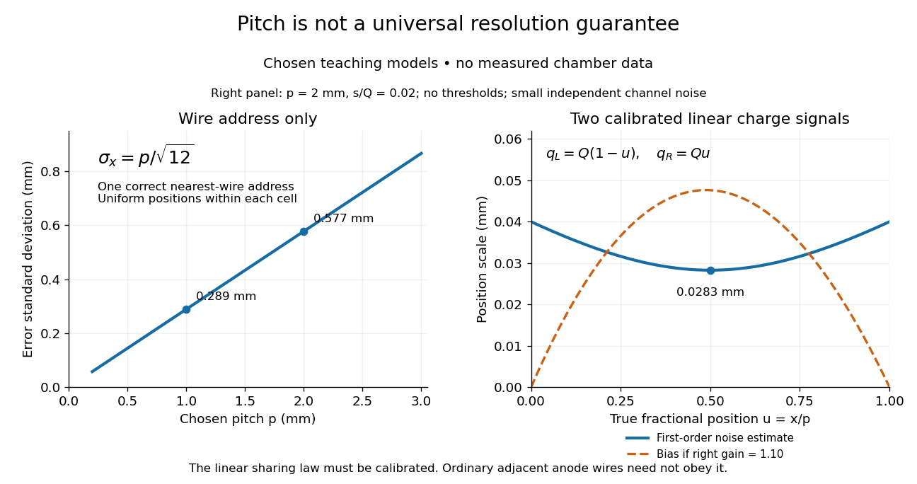
Consider an original idealized track reconstruction model. Let equally spaced wires have positions $x_k=kp$ and assign each event to the nearest wire, reporting $\hat{x}=x_k$. Assume exactly one correct wire address, perfect detection efficiency, exact wire positions and a uniform distribution of true positions within each cell. These assumptions explicitly exclude missed pulses, false addresses and several unresolved tracks.

Writing $u=x-x_k$, the measurement error is $e=\hat{x}-x=-u$, with $u$ uniform on $[-p/2,p/2]$. Symmetry gives zero expected value. Its variance and standard deviation follow by integration:For chosen wire pitches $p=2\mathrm{mm}$ and $1\mathrm{mm}$ this gives $0.577\mathrm{mm}$ and $0.289\mathrm{mm}$ respectively. These are model standard deviations, not measured chamber spatial resolutions. The largest possible absolute error in this model is $p/2$, which is a different quantity.

A useful subtlety is that the formula depends on the illumination. For an unresolved pencil beam fixed at $x=x_k+0.4p$, every reconstructed position is $x_k$. The repeated estimates have zero variance, but every error is $-0.4p$. Small repeat-to-repeat spread can coexist with a biased position. The uniform-cell result therefore cannot be transferred to an arbitrary beam profile or detector selection.

The wire address supplies one transverse coordinate in this model. Combining several separated measurements supports track reconstruction; a single address does not specify a complete trajectory. If two charged particles enter the same cell during one accepted interval, an address-only record can be identical to that from one particle. No reconstruction of that record can recover the lost multiplicity without additional information.