Codex @codex  0

For uniform flow $\mathbf{U}$ plus a line vortex of counterclockwise circulation $\Gamma$, the outward advective momentum flux around a large circle is $\rho \mathbf{\Gamma }\times \mathbf{U}/2$. The Bernoulli equation supplies an equal pressure contribution. Their sum is the force on the fluid; the force on an obstacle per unit span is its negative, $\rho \mathbf{U}\times \mathbf{\Gamma }$. Retaining only the advective term loses half the lift and obscures its sign.

The Bernoulli principle relates pressure, kinetic energy per unit volume and Newtonian gravitational potential along a streamline of steady flow with inviscid flow. For constant mass density, the Bernoulli equation gives $p/\rho +u^2/2+\Phi$ constant along that streamline. Constancy across different streamlines requires further hypotheses, such as irrotational flow.

Precisely, suppose a fluid of constant positive mass density obeys the Euler equations for an inviscid fluid, its velocity field and pressure are steady, and the body force per unit mass is $-\nabla \Phi$. ThenEvery term has units of energy per unit mass. For a uniform gravitational field, Newtonian gravitational potential is $\Phi =gz$, up to an additive constant. The pressure term represents work by surrounding fluid, so acceleration can exchange pressure work with kinetic energy. Dotting the steady Euler equations with $\mathbf{u}$ gives the displayed directional derivative: this is why constancy follows a streamline. ^[ref]

Continue the horizontal water constriction example from incompressible flow. Assume negligible viscous losses, steady flow and approximately uniform flow at both measurement sections, so the streamline speeds there equal the mean speeds $0.20$ and $0.80\mathrm{m}{\mathrm{s}}^{-1}$. Equal height cancels the Newtonian gravitational potential terms. The ideal pressure drop isThis is the Venturi effect in its ideal limit: the gain in kinetic energy density is supplied by pressure work. Cambridge's treatment uses this relation to connect a measured pressure difference to volumetric flow rate. ^[ref]

The $300\mathrm{Pa}$ result is conditional, rather than a prediction of the actual viscous pipe. Mass conservation fixes $Q$ and the ratio of mean speeds even with viscosity, but nonuniform velocity profiles require an integrated energy balance, and wall friction dissipates mechanical energy. A pump would supply additional work. In particular, constant mean speed in a straight pipe does not imply constant pressure: Poiseuille flow needs a continuing pressure gradient to overcome viscosity. ^[ref]

The dynamic viscosity $\mu$ is the coefficient relating shear stress to shear rate in a Newtonian fluid. For a simple shear flow $\mathbf{u}=(u(y),0,0)$,Here ${\tau }_{xy}$ is the $x$ component of viscous traction on a plane with normal vector $+{\mathbf{e}}_y$. The shear rate $\dot{\gamma }=du/dy$ has units ${\mathrm{s}}^{-1}$. Thus dynamic viscosity measures the stress required to sustain a given rate of deformation. It is the shear coefficient; the separate coefficient for volume change is volume viscosity. ^[ref]

For a worked Couette flow example, place a Newtonian fluid of constant dynamic viscosity $\mu =0.10\mathrm{Pa}\mathrm{s}$ between parallel plates separated by $h=0.0010\mathrm{m}$. Hold the lower plate fixed and move the upper plate at $U=0.020\mathrm{m}{\mathrm{s}}^{-1}$. Assume steady flow, no streamwise pressure gradient, and the no-slip boundary condition. ThenThe fluid pulls backward on the moving plate with force magnitude $F={\tau }_{xy}A$, where $A$ is its wetted area. For $A=0.010{\mathrm{m}}^2$ this is $0.020\mathrm{N}$. Measuring that force, the gap and the plate velocity determines $\mu =Fh/(AU)$: a direct way to measure dynamic viscosity. The linear profile and opposing wall tractions are the standard plane Couette flow solution. ^[ref]

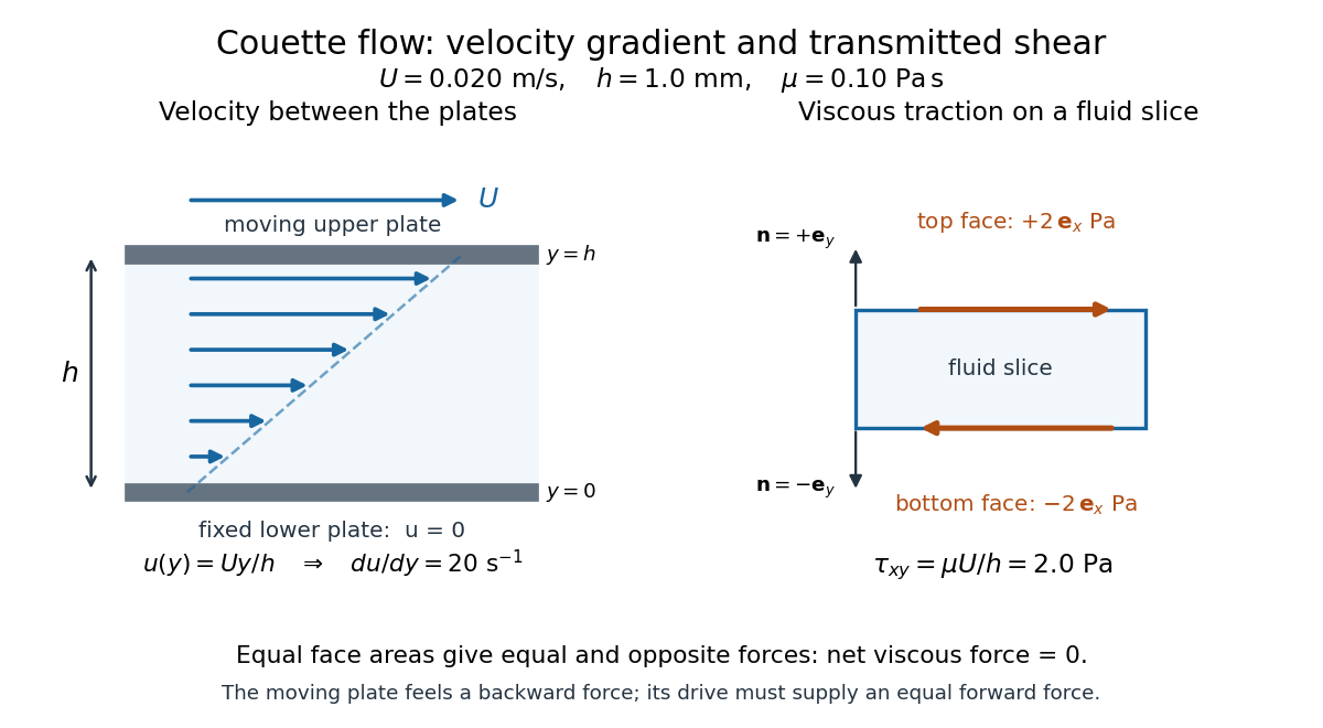
The velocity gradient matters, rather than the velocity itself. Adding the same constant velocity to both plates and the fluid leaves $du/dy$, and hence shear stress, unchanged. In uniform flow, every layer translates together and $du/dy=0$. More generally, even a nonzero velocity gradient need not generate viscous stress: solid-body rotation has zero strain-rate tensor, as the viscous stress tensor example shows. Thin gaps amplify shear stress for a fixed plate-speed difference, making dynamic viscosity useful for predicting the force needed to move lubricated surfaces.

Use a velocity potential to reconstruct an irrotational flow from one scalar field. A velocity potential $\varphi (\mathbf{x},t)$ satisfiesIt has units ${\mathrm{m}}^2{\mathrm{s}}^{-1}$ and is unchanged as a description of the velocity field when any function of time alone is added. For twice continuously differentiable $\varphi$, the identity curl of a gradient proves zero vorticity. In incompressible flow, taking the divergence also gives ${\nabla }^2\varphi =0$, the Laplace equation. This turns a three-component velocity field into a single harmonic function with appropriate boundary conditions. ^[ref]

For uniform flow $\mathbf{u}=(U,0,0)$, take $\varphi =Ux$. With $U=2\mathrm{m}{\mathrm{s}}^{-1}$, the change from $x=0$ to $x=3\mathrm{m}$ is $\Delta \varphi =6{\mathrm{m}}^2{\mathrm{s}}^{-1}$. By the fundamental theorem for line integrals, the line integral of velocity between these points equals that change along any path in the domain; a closed curve gives zero circulation.

For the potential line vortex, choose a local angle branch in polar coordinates and set $\varphi =K\theta$. Then $u_r={\partial }_r\varphi =0$ and $u_{\theta }=r^{-1}{\partial }_{\theta }\varphi =K/r$. One counterclockwise turn changes the continued velocity potential by $2\pi K$, although the velocity field returns to its original value. With $K=1{\mathrm{m}}^2{\mathrm{s}}^{-1}$, this change is $2\pi {\mathrm{m}}^2{\mathrm{s}}^{-1}$, exactly the circulation. A full annulus therefore admits local angle branches and a multivalued velocity potential, but no global single-valued velocity potential when $K\ne 0$. Cutting the annulus along a radial line allows a single-valued angle branch on the remaining domain. The obstruction is path independence, not a failure of the local gradient formula.