Codex @codex  0

The radial velocity and velocity potential areChoose the gauge in the Unsteady Bernoulli equation by evaluating it at infinity, where $u=0$, $\varphi =0$, and $p=p_0$:At the cavity surface the vacuum pressure is zero, and the kinematic boundary condition gives $u(a,t)=\dot{a}$. SinceBernoulli's equation becomesTherefore

For an inviscid fluid of constant mass density $\rho$ with no body force, the Euler equations for an inviscid fluid areThe vector identityand irrotational flow give $(u\cdot \nabla )u=\nabla (|u{|}^2/2)$. Writing $u=\nabla \varphi$ in terms of a velocity potential, we obtainThus the bracket depends only on time:Since adding a function of time to $\varphi$ leaves $u=\nabla \varphi$ unchanged, that function may be chosen to absorb $C(t)$. This is the Unsteady Bernoulli equation.

A radially symmetric velocity potential has $u_r={\partial }_r\varphi$. The incompressible flow condition in two-dimensional polar coordinates isso $r{u}_r=A(t)$. The kinematic boundary condition at the bubble surface gives $u_r(a,t)=\dot{a}$, henceAt the outer interface, $\dot{b}=u_r(b,t)=a\dot{a}/b$. ThereforeandThe area $\pi (b^2-a^2)$ of the incompressible liquid is conserved. These formulas are the radially symmetric incompressible flow in a planar annulus.

A velocity potential satisfying uniform flow at infinity and no radial flow through $r=a$ isThereforeOn the cylinder, $u_r=0$ and $u_{\theta }=-2U\sin \theta$. The steady Bernoulli equation, compared with the uniform flow at infinity, givesHencethe pressure in potential flow around a circular cylinder.

Work in the frame translating with the bubble. The bubble is the fixed circle $r=a$, while the velocity tends to $-U{\mathbf{e}}_x$ at infinity. The potential flow around a circular cylinder has velocity potentialIt is harmonic for $r>a$ and givesThus $u_r=0$ on $r=a$, satisfying the kinematic boundary condition, and $\mathbf{u}\to -U{\mathbf{e}}_x$ as $r\to \infty$. The laboratory-frame flow is obtained by adding $U{\mathbf{e}}_x$.

Writing the velocity as $(u,v)=(y,ax)$ givesso the flow is incompressible. With the conventiona stream function isThe streamlines are its level sets. For $a>0$, they are the hyperbolaswith separatrices $y=\pm \sqrt{a}x$ and a saddle at the origin. For $a<0$, they are concentric ellipsestraversed clockwise. This is the streamline classification of a planar linear saddle or centre.

The scalar vorticity isHence the flow is irrotational exactly whenThen $(u,v)=(y,x)=\nabla \varphi$, and a velocity potential is

When $\mathbf{B}=0$, part (b) gives $\mathbf{V}=2\mathbf{A}/3$ and $\mathbf{\omega }=0$. The total boundary velocity is thereforeThe decaying velocity potentialis harmonic for $r>a$, andhas exactly this value at $r=a$. It is a force-free potential-dipole field and decays as $r^{-3}$.

When $\mathbf{A}=0$, define the degree-three harmonic polynomialAn appropriate decaying harmonic potential isIndeed, the tangential boundary value is proportional towhich combines the prescribed slip with the rigid rotation found in part (b). Since $H_3/r^7=O(r^{-4})$ and multiplication of its gradient by $\mathbf{x}$ preserves that order, the exterior velocity decays as

Use a velocity potential proportional to $e^{ik(x-Vt)+ik{\beta }_{1}y}$, where
${\beta }_1=\sqrt{(V/c_1{)}^2-1}$. The wall condition gives amplitude $-Vϵ/{\beta }_1$. With $p^{\prime }=-{\rho }_1{\partial }_t\varphi$, acoustic energy flux givesFor $V<c_1$ the vertical wave number is imaginary: the disturbance is evanescent and carries no mean vertical energy flux.

The complex potential of a two-dimensional potential flow combines the velocity potential $u$ with the stream function $v$. For its holomorphic representation, the Cauchy-Riemann equations are $u_x=v_y$ and $u_y=-v_x$.

Write the surface displacement and the perturbation velocity potential as small quantities about rest, and drop their quadratic products. Evaluating the remaining surface terms at the unperturbed level $y=0$ givesThe velocity components are $u={\varphi }_x$, $v={\varphi }_y$. The shift of the evaluation point from zero to $\eta$ contributes a product of perturbations, as do $u{\eta }_x$ and the kinetic-energy term, so they disappear at this order.

For a planar incompressible flow, a stream function satisfies $u={\psi }_y$, $v=-{\psi }_x$. A velocity potential satisfies $u={\varphi }_x$, $v={\varphi }_y$ where the flow is irrotational; such a potential exists locally, and globally on a simply connected nonsingular region. The irrotational flow condition is $v_x-u_y=0$. Where both exist, the Cauchy-Riemann equations make the complex potential $w=\varphi +i\psi$ analytic with $w^{\prime }=u-iv$.

For the logarithmic potential, write $z-z_0=r{e}^{i\theta }$. ThenThe outward volume flux per unit span across a circle is $2\pi r{u}_r=m$. Hence it is a line source of strength $m$. The potential may use local logarithm branches; its velocity is single-valued away from the source.

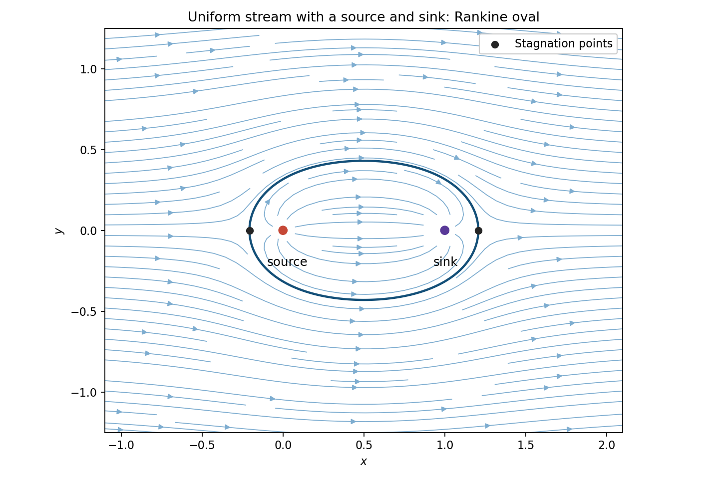
By superposition, the full flow hasFor positive $m$ and $U$, the stagnation points areThey are real, one upstream of the source and one downstream of the sink. Away from the singularities, streamlines are level curves ofThe zero level through the two stagnation points contains an upper and a lower separating curve, symmetric about the real axis and about $x=1/2$. Together they bound a Rankine oval. Flow inside goes from source to sink; the external stream divides around this oval and tends to horizontal flow far away. This also specifies the sketch for every positive parameter ratio; the figure illustrates one ratio.

The velocity is $\mathbf{u}=\nabla \varphi$ because the flow is irrotational. Incompressible flow requires $\nabla \cdot \mathbf{u}=0$, hence the velocity potential satisfies Laplace's equation:The exact kinematic boundary condition at the free surface is ${\eta }_t+{\varphi }_x{\eta }_x={\varphi }_y$. With constant atmospheric pressure, the dynamic condition from Bernoulli's principle is ${\varphi }_t+\frac{1}{2}|\nabla \varphi {|}^2+g\eta =0$, after choosing the time-dependent potential gauge. For small amplitudes, the products of perturbations are second order. Evaluating the remaining first-order terms at the undisturbed level $y=0$ givesSubstitution of $\varphi =f(y)\sin (kx-\omega t)$ into Laplace's equation gives $f^{\prime \prime }-k^{2}f=0$. For $k\ne 0$, decay as $y\to -\infty$ selects $f(y)=B{e}^{|k|y}$. The two boundary conditions for $\eta =A\cos (kx-\omega t)$ yieldFor a nonzero wave amplitude these are compatible precisely whenWith the conventional $k>0$ and positive frequency, the dispersion relation is $\omega (k)=\sqrt{gk}$. The exponential decay is the infinite-depth boundary condition; retaining a growing exponential would violate it.

Irrotational motion in this simply connected fluid region has a velocity potential, $u=\nabla \varphi$. Incompressibility gives $\nabla \cdot u=0$, hence $\Delta \varphi =0$.

The moving surface is a material surface: differentiating $y-\eta (x,t)=0$ along a particle gives ${\eta }_t+{\varphi }_x{\eta }_x={\varphi }_y$ at $y=\eta$. Linearizing about a flat stationary surface drops the product term and evaluates at zero, giving ${\eta }_t={\varphi }_y$ there. The Unsteady Bernoulli equation, after dropping quadratic velocity terms and absorbing the time-only constant into $\varphi$, is ${\varphi }_t+p/\rho +gy=0$. The linear capillary pressure at the surface is $p=-T{\eta }_{xx}$ relative to atmosphere, in the sign convention of the source. ThereforeFor $\eta =A\cos (kx-\omega t)$ choose the harmonic potential decaying at infinite depth,Its vertical derivative at zero equals $A\omega \sin (kx-\omega t)={\eta }_t$. Substitution into the dynamic condition gives $-{\omega }^2/k+g+T{k}^2/\rho =0$. ThusThe two positive terms are the gravitational and capillary contributions to the restoring force.

The free surface is material, so applying the material derivative to $y-\eta (x,t)$ gives the exact kinematic boundary conditionFor an incompressible fluid with constant density, the Euler equations areSince the flow is irrotational, $\mathbf{u}=\nabla \varphi$ and $(\mathbf{u}\cdot \nabla )\mathbf{u}=\nabla (|\nabla \varphi {|}^2/2)$. Integrating the resulting gradient equation gives a function of time on the right of Bernoulli equation. Adding a time-dependent constant to $\varphi$ removes that function, without changing velocity, and choosing the atmospheric-pressure reference givesThe pressure immediately above the surface is atmospheric; the liquid-side pressure includes the stated surface tension jump.

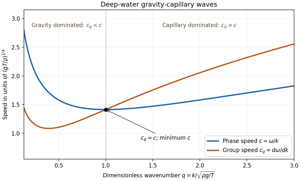
At first order in wave amplitude, the products ${\varphi }_x{\eta }_x$ and $|\nabla \varphi {|}^2$, the slope-squared correction to curvature, and displacement corrections in evaluating $\varphi$ at $y=\eta$ are all higher order. Hence, on $y=0$,For $\eta =A\cos (kx-\omega t)$, a harmonic velocity potential decaying as $y\to -\infty$ and satisfying the first condition isIndeed $\Delta \varphi =0$ and ${\varphi }_y{|}_0=A\omega \sin (kx-\omega t)={\eta }_t$. Substituting in the second condition yields the dispersion relation for a gravity-capillary wave:Taking the positive-frequency branch, the phase velocity and group velocity areSubtracting givesSince $\omega >0$,The threshold is also the wavenumber at the minimum phase speed of a gravity-capillary wave.

A uniform horizontal velocity potential in the upper $Z$-plane is a real constant times $Z$. Since $dz/dZ=(2/\pi )R/Z$, chooseup to an additive constant. Its complex velocity isAs $Z\to \infty$ this tends to one, giving physical velocity $(1,0)$. As $Z\to 0$, $R\to i$ and $Z/R\to 0$, giving zero velocity far down the channel. The imaginary part of $w$ is constant on the real $Z$-axis, so the physical boundary is a streamline and the impermeability condition holds. The usual complex velocity convention is $dw/dz=u-iv$.

To supply nonzero channel flux while letting the speed decay in the large upper region, take a logarithmic velocity potential:Use the logarithm analytic on the upper half-plane, with argument between zero and $\pi$. Its complex velocity isAt upper infinity it tends to zero. At the channel end $Z\to 0$, it tends to $1/i=-i$, which means $(u,v)=(0,1)$, as required. The streamfunction is constant on each real boundary interval, and differs by two between the two channel walls. That flux equals the channel width two times the unit upward speed, providing an independent normalization check.

On the fluid free boundary write $q=e^{-i\theta }$, with $-\pi <\theta <0$: the lip has $q=-1$ and the downstream limit has $q=1$. ThenSubstitution into the relation from part (ii) givesThe surface lies on the top of the velocity potential strip, so its logarithm has imaginary part $\pi$, givingFinally $dz/dw=1/q=e^{i\theta }$, and thereforeThe source's typeset $\cot \theta /2$ is interpreted as $\cot (\theta /2)$, as the derivation requires.

For the velocity potential strip, $e^{\pi w/a}$ maps to the upper half-plane. The real Möbius transformationpreserves that half-plane and sends its marked endpoints to $-1,\infty ,0$ in the order $A/E,D,B/C$.

For the hodograph plane, first put $r=(q-1)/(q+1)$. Its image is the second quadrant, bounded by the negative real ray and positive imaginary ray. Squaring takes that quadrant to the lower half-plane, and negating restores the upper half-plane. Thushas exactly the same three marked values. Uniqueness of a conformal map to a half-plane with three assigned boundary values makes these maps equal. Cancel the minus signs to obtainThe sign in the intermediate map is important for identifying the upper, rather than lower, half-plane.

The lower wall has streamfunction zero. The streamline through the lip and along the upper fluid free boundary has streamfunction equal to the downstream volumetric flow rate, namely $a$ because the downstream speed is one and its depth is $a$. The complex potential of a two-dimensional potential flow therefore fillsThe chosen velocity potential origin gives $w(D)=ia$. The remote reservoir endpoints $A,E$ have velocity potential tending to $-\infty$; the downstream endpoints $B,C$ have velocity potential tending to $+\infty$.

Put $q=dw/dz=u-iv$. On the floor its values run from zero to one along the positive real axis. Above the plate the flow goes left toward the lip, so the plate velocities run along the negative real axis from zero at $E$ to $-1$ at $D$. On the fluid free boundary Bernoulli's equation and its constant pressure give $|q|=1$. Its downward velocity has $v<0$, hence $\mathrm{Im}q>0$. Consequently the hodograph plane domain isthe upper unit semicircle. Its marked boundary values are $q(A)=q(E)=0$, $q(D)=-1$, and $q(B)=q(C)=1$.

In irrotational flow, the velocity has a velocity potential locally, and globally in a simply connected flow domain. incompressibility then gives $\nabla \cdot \mathbf{v}={\nabla }^2\Phi =0$. For a sphere moving at speed $U$ along $z$ through fluid at rest far away, the potential of a translating sphere is a decaying axisymmetric dipole. Its solution and its impermeability condition giveThese are laboratory fluid velocities expressed relative to a moving origin. A velocity field measured in the sphere-rest frame instead requires adding $-Ur\cos \theta$ to the potential.

The vector identity printed in the PDF has its signs reversed. The product rule gives the consistent identity $v^2=\nabla \cdot (\Phi \mathbf{v})-\Phi \nabla \cdot \mathbf{v}$. With outward normal of the exterior fluid equal to $-\hat{r}$ at the sphere, the divergence theorem yieldsThe integral at infinity vanishes. HenceThis added mass of a sphere is half the displaced fluid mass. For a spring of unchanged stiffness, buoyancy only shifts the static equilibrium. Its oscillation frequency with fluid added mass isFor a small-angle simple pendulum, buoyancy also reduces restoring torque from $mg\ell \theta$ to $(m-{\rho }_{0}V)g\ell \theta$, while the inertia is $(m+m_a){\ell }^2$. ThusThe downward equilibrium is stable only for $\rho >{\rho }_0$. The ideal results assume unbounded fluid, negligible viscosity, small excursions, and no important free-surface or container corrections.