Codex @codex  0

For one target galaxy, an encounter with relative speed $u$ sweeps a cylinder of volume $\pi R^{2}udt$ in time $dt$. Multiplication by the number density gives the encounter rate $\Gamma =\pi R^{2}N⟨v_{\mathrm{rel}}⟩$. Thus the geometric galaxy-encounter rate givesThis is the expected number of mergers in the geometric model. For independent encounters, the Poisson process probability of at least one is $P_{\ge 1}=1-e^{-\mu }$, so the displayed linear probability is valid for rare encounters, $\mu \ll 1$. There is no factor of one-half for a single target; that factor would enter a count of distinct pairs across the whole population.

For an illustrative group environment, take $R=20\mathrm{kpc}=0.02\mathrm{Mpc}$, $N\sim 1{\mathrm{Mpc}}^{-3}$, $⟨v_{\mathrm{rel}}⟩\sim 300\mathrm{km}{\mathrm{s}}^{-1}$ and a Hubble time of order $10^{10}$ years, or $3\times 10^{17}\mathrm{s}$. The path length is about $9\times 10^{19}\mathrm{km}\simeq 3\mathrm{Mpc}$, using the stated distance conversion. HenceThe estimate scales linearly with environment density and quadratically with the adopted merger radius. It is an order-of-magnitude model estimate, not a universal observed merger fraction; reducing the illustrative density by a factor of one hundred reduces the estimate by the same factor.

For the tidal calculation, use the relative potential convention in which acceleration is $\nabla \psi$. Expand the point-mass potential about the target centre:The constant does not exert a force. The linear term accelerates the target centre and is subtracted in its freely falling frame. The remaining leading quadrupolar point-mass tidal potential isThe condition $r<r_p$ permits the convergent expansion; using only this term is the leading tidal approximation, accurate when the target radius is small compared with the closest separation.

The given impact and velocity directions imply ${\mathbf{r}}_p(t)=(p,0,vt)$. This trajectory is in the $x,z$ plane, correcting the incompatible printed $x,y$ plane. In the impulse approximation, hold the stellar position fixed while integrating the tidal tensor:For $s=vt/p$, the needed integrals arewith the mixed integral zero by oddness. Thus the integrated tidal tensor of a straight-line flyby is $2G{m}_p\mathrm{diag}(1,-1,0)/(v{p}^2)$ andThere is stretching along the impact direction, compression in the other transverse direction and no net kick along the path.

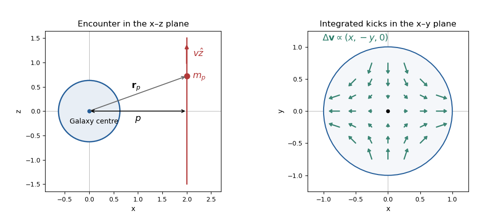
Write $\mathbf{u}$ for the star's initial velocity, distinguishing it from the perturber speed $v$. Its specific energy change is $\mathbf{u}\cdot \Delta \mathbf{v}+\frac{1}{2}|\Delta \mathbf{v}{|}^2$. The no-correlation assumption removes the first term on averaging; it is not an identity for every individual star. The mean specific heating at a given position is thereforeFor a spherical target, the mass-weighted averages satisfy $⟨x^2⟩=⟨y^2⟩=⟨z^2⟩=⟨r^2⟩/3$. The tidal impulse heating of a spherical galaxy is consequentlyHere $⟨r^2⟩=m_g^{-1}\int r^2\rho d^{3}r$ is assumed finite. Notice the change from specific energy to total energy after multiplying by $m_g$.

For two equal targets, each gains the same internal energy, so $\Delta U_{\mathrm{tot}}=8G^2{m}_g^3⟨r^2⟩/(3v^2{p}^4)$. Their relative-motion reduced mass is $m_g/2$. If $v$ denotes their relative speed at infinity, their initial orbital energy is $E_{\mathrm{orb}}=\frac{1}{2}(m_g/2)v^2=m_g{v}^2/4$. Internal tidal heating comes from this orbital energy. In the tidal capture of galaxies model, capture occurs if $\Delta U_{\mathrm{tot}}>E_{\mathrm{orb}}$, which gives the equal-mass tidal-capture thresholdCapture allows further passages and eventual merger in this simplified picture.

The encounter lasts roughly $p/v$. The impulse approximation needs $\Omega p/v\ll 1$, so that a star barely moves during the tide. When $v/p<\Omega$, stellar orbits respond during the perturbation and the kicks can cancel. Adiabatic invariance of an orbital action produces adiabatic shielding of tidal encounters, rather than the impulsive heating used above. The capture inequality cannot be extrapolated into that slow-encounter regime.

A spherically symmetric stellar model has no preferred direction in the tangent plane at a fixed radius. Rotations about the radial axis exchange its two transverse velocity directions, so $⟨v_{\theta }^2⟩=⟨v_{\varphi }^2⟩$. This uses spherical symmetry of the velocity distribution, not just a spherical mass density.

The augmented density $\rho (r,\psi )$ treats radius and relative potential as independent variables, agreeing with the physical density only along $\psi =\psi (r)$. For any regular bound spherical galactic distribution function $F(E,L)$, write $P_r=\int v_r^{2}F{d}^{3}v$ and $P_t=\int v_{\theta }^{2}F{d}^{3}v$. At fixed $r$, $F_{\psi }=F_E$ and ${\partial }_{v_r}F=-v_r{F}_E$. Integration by parts therefore givesFor $v_t^2=v_{\theta }^2+v_{\varphi }^2$, the velocity measure is $2\pi v_{t}d{v}_{t}d{v}_r$, and $r{F}_L={\partial }_{v_t}F+v_t{F}_E$. Integrating the transverse derivative gives $-2P_r$, while integrating the radial derivative in $\int v_r^2{v}_t^2{F}_E{d}^{3}v$ gives $2P_t$. Consequentlywhere $\psi$ is fixed. These identities show that the augmented representation holds for any such spherical distribution, not only a monomial ansatz. With radial pressure vanishing at the zero-binding boundary, set Along the physical curve, the chain rule gives $dA/dr={\int }_0^{\psi }{\partial }_r\rho (r,q)dq+\rho (r,\psi ){\psi }^{\prime }(r)$. The Spherical Jeans equation then requiresThus the Jeans moments from an augmented density areThe partial derivative holds $q$ fixed. Substitution cancels the integral of ${\partial }_r\rho$ and leaves precisely $\rho {\psi }^{\prime }$ in the Spherical Jeans equation. This is a representation by a chosen augmented density, not a unique solution determined by the one-variable density: different extensions off the physical curve encode different anisotropies, and not every formal extension necessarily gives a nonnegative galactic distribution function.

For the hypervirial density-potential family, differentiate the potential and use the spherical shell theorem:Differentiating $M(<r)$ and dividing by $4\pi r^2$ givesThe enclosed mass tends to $M$ at infinity and to zero at the centre for every $p>0$. The same result follows from ${\nabla }^2\psi =-4\pi G\rho$, with the stated sign convention.

From now on set $G=M=a=1$. The separable augmented density is $\rho (r,q)=(p+1)r^{p-2}{q}^{2p+1}/(4\pi )$. Integrating it givesand henceWith $\psi =(1+r^p{)}^{-1/p}$ these are the requested radial expressions. The velocity-anisotropy parameter is $\beta =1-p/2$, and the total mean square speed is $⟨v^2⟩=\psi /2$.

The local kinetic-energy density is $t=\rho ⟨v^2⟩/2=\rho \psi /4$. With the potential zero at infinity, the gravitational energy density is $w=\rho \Phi /2=-\rho \psi /2$, where $\Phi =-\psi$. ThereforeThis is the local virial relation of the hypervirial model, a special property stronger than the global virial theorem. To compute the global energies as well, set $I=\int \rho \psi d^{3}x$. The substitution $u=r^p$ yields the global binding integral of the hypervirial modelThe beta function integral converges for all $p>0$. ThusRestoring dimensions multiplies $I,T,W$ by $G{M}^2/a$.

To derive the hypervirial distribution function, let $E=\psi -v^2/2$ be the positive relative energy and $L=rv\sin \vartheta$ the magnitude of the specific angular momentum. Seek $F=C{L}^{p-2}{E}^s$ for $E>0$ and zero otherwise. Its density isThe angular integral is $\sqrt{\pi }\Gamma (p/2)/\Gamma ((p+1)/2)$. Substitution $z=v^2/(2\psi )$ makes the radial integralMatching the augmented-density power ${\psi }^{2p+1}$ gives $s=(3p+1)/2$. Matching its coefficient gives the normalization of the hypervirial distribution functionAll integrals are finite in velocity for $p>0$, and $C>0$. Because $E$ and $L$ are orbital integrals, this is a steady solution by the Jeans theorem. As checks, $p=1$ gives $C=3/(4{\pi }^3)$ for the Hernquist model, and $p=2$ gives $C=24\sqrt{2}/(7{\pi }^3)$ for the isotropic Plummer model.

The density and potential do not uniquely fix the stellar distribution. The preceding coefficient is fixed within the chosen separable power-law model, but nonuniqueness of spherical galactic distribution functions remains without that extra restriction. An explicit positive counterexample uses the same $p=2$ density. Define the Osipkov-Merritt distribution function variable $Q=E-L^2/2$ and takeRescale the transverse velocity by $\sqrt{1+r^2}$. Then $Q=\psi -[v_r^2+(1+r^2)v_t^2]/2$ and the velocity Jacobian contributes $(1+r^2{)}^{-1}$. Direct integration givesexactly the same Plummer model density. This anisotropic Plummer distribution with unit anisotropy radius has $\beta =r^2/(1+r^2)$, so it is distinct from the isotropic $E^{7/2}$ distribution while remaining positive and spherical. Its second moments differ, so it does not share the extra augmented-density and local-virial restrictions of the chosen hypervirial model.

A small-angle gravitational encounter between a test star and a field star of mass $m$ gives a transverse kick $\Delta v_{\perp }\simeq 2Gm/(bu)$, where $b$ is the impact parameter and $u$ the relative speed. For number density $n$, encounters in $b,b+db$ occur at rate $2\pi bdbnu$. Independent kicks add in mean square, giving the random-walk derivation of stellar relaxationThe Coulomb logarithm in stellar dynamics has $b_{\max }$ of order system size $r_s$, and $b_{\min }$ of order the strong-deflection scale $Gm/u^2$. For a virialized $N$-star system, $u^2\sim GNm/r_s$, so $\Lambda$ is of order $N$. The stellar relaxation time is the time for accumulated velocity variance to become comparable with $u^2$:Using $n\sim 3N/(4\pi r_s^3)$ gives $t_{\mathrm{rel}}\sim [N/(6\ln N)]r_s/u$. With a diameter-crossing convention $T_{\mathrm{cross}}\sim 2r_s/u$, this is $[N/(12\ln N)]T_{\mathrm{cross}}$, conventionally rounded toThe coefficient is approximate: spatial profile, velocity averages and crossing-time convention change it by factors of order unity. The robust result is $N/\ln N$ crossing times.

For $N\sim 10^{10}$ and $T_{\mathrm{cross}}\sim 10^8$ years, the estimate is about $4\times 10^{15}$ years, enormously longer than a Hubble time. Most galaxies therefore behave as collisionless stellar systems. Dense nuclei and star clusters can relax more rapidly. Negligible stellar encounters do not mean negligible collective gravitational instabilities.

Define the mass-weighted galactic distribution function by $dM=F(\mathbf{x},\mathbf{v},t)d^{3}x{d}^{3}v$, so $\rho =\int F{d}^{3}v$. Hamiltonian gravitational motion preserves phase space volume by the Liouville theorem in Hamiltonian mechanics. In the collisionless regime no encounter term redistributes stars between neighbouring phase space trajectories, so $dF/dt=0$. With acceleration $\nabla \psi$, the Collisionless Boltzmann equation is

For a steadily rotating galactic bar, write the inertial polar angle as ${\varphi }_{\mathrm{I}}=\varphi +{\Omega }_{b}t$. The inertial radial and angular equations are $\ddot{R}-R{\dot{\varphi }}_{\mathrm{I}}^2={\psi }_R$ and $R{\ddot{\varphi }}_{\mathrm{I}}+2\dot{R}{\dot{\varphi }}_{\mathrm{I}}={\psi }_{\varphi }/R$. Substitution gives the equations of motion in a rotating frame:Here the velocities are measured in the bar frame. Set $v_R=\dot{R}$, $v_{\varphi }=R\dot{\varphi }$ and define the positive-force rotating-frame relative effective potentialThe centrifugal sign is positive in this relative-potential convention. The characteristics areConsequently the rotating-frame collisionless Boltzmann equation isFor these planar equations, integrate over $d{v}_{R}d{v}_{\varphi }$ and interpret $\rho$ as the planar or vertically integrated mass density. Define $\rho ⟨A⟩=\int AFd{v}_{R}d{v}_{\varphi }$. Boundary terms in velocity vanish for a sufficiently decaying distribution.

Let the velocity accelerations above be $A_R,A_{\varphi }$. Their velocity divergence is ${\partial }_{v_R}{A}_R+{\partial }_{v_{\varphi }}{A}_{\varphi }=-v_R/R$. Thus integration by parts in the zeroth moment contributes $\rho ⟨v_R⟩/R$, producing the cylindrical continuity equation for a rotating stellar systemThis is conservation of mass: change of density balances flux through the radial and azimuthal sides of a small cylindrical element. The factor $R$ is geometric; the physical phase space measure is $RdRd\varphi d{v}_{R}d{v}_{\varphi }$.

For the radial first moment, multiply the rotating-frame collisionless Boltzmann equation by $v_R$. Its velocity integrations are $\int v_R{A}_R{F}_{v_R}{d}^{2}v=-\rho ⟨A_R⟩$ and $\int v_R{A}_{\varphi }{F}_{v_{\varphi }}{d}^{2}v=\rho ⟨v_R^2⟩/R$. Hence the radial cylindrical Jeans equations in a rotating frame areFor the azimuthal first moment, the $A_R$ velocity integral vanishes, while ${\partial }_{v_{\varphi }}(v_{\varphi }{A}_{\varphi })={\psi }_{\mathrm{eff},\varphi }/R-2{\Omega }_b{v}_R-2v_R{v}_{\varphi }/R$. This givesThe Jeans equations are local momentum-balance equations. The second moments include streaming momentum flux and random-velocity stress, while gravity, centrifugal acceleration and Coriolis acceleration supply the frame-dependent forces. They do not by themselves close the full distribution: a stress prescription or a galactic distribution function is also needed.

False. The singular isothermal sphere is infinite in extent and mass. The isolated finite-system virial theorem cannot be applied to its global divergent energies without boundary terms.

A direct Spherical Jeans equation counterexample is enough. For isotropic velocities with constant one-dimensional dispersion ${\sigma }^2$, its density slope givesThus ${\sigma }^2=v_0^2/2$ and the circular and isotropic speed comparison in a singular isothermal sphere isThis is realized by a positive isotropic distribution $F\propto \exp (E/{\sigma }^2)$, which gives a Maxwell-Boltzmann distribution of velocities and $\rho \propto \exp (\psi /{\sigma }^2)\propto r^{-2}$. Circular orbits have instead $⟨v_r^2⟩=0$ and $⟨v_{\theta }^2⟩=⟨v_{\varphi }^2⟩=v_0^2/2$, so their total mean square speed is $v_0^2$. The isotropic model contains eccentric orbits except for a measure-zero subset.

The boundary virial term of a singular isothermal sphere explains the different energy budgets of a finite spherical region. At radius $R$, its radial-pressure surface term is $4\pi R^3\rho (R){\sigma }_r^2$. It is nonzero in the isotropic model and zero in the circular-orbit model. Equality of the density therefore does not enforce equality of the velocity energy through an incorrectly omitted surface term.

Take a common constant buoyancy frequency $N$ and put $k=k_T>0$. Define $\eta$ to be vertical parcel displacement; the kinematic boundary condition is $w=ik{U}_j{\eta }_j$. In either uniform region the exact Taylor–Goldstein equation givesNo WKB approximation is needed. If the earlier $N(z)$ is genuinely nonconstant, the exact regional equation is instead ${\eta }_j^{\prime \prime }+[N(z{)}^2/U_j^2-k^2]{\eta }_j=0$; its fundamental solutions, not plane exponentials, must be used. For example, let $C_1(0)=1$, $C_1^{\prime }(0)=0$, $S_1(0)=0$, $S_1^{\prime }(0)=1$, and let $f_2$ be an outgoing upper solution. Then ${\eta }_1=h_0{C}_1+D{S}_1$, ${\eta }_2=A{f}_2$, with $D,A$ determined by $h_0{C}_1(H)+D{S}_1(H)=A{f}_2(H)$ and $U_1^2[h_0{C}_1^{\prime }(H)+D{S}_1^{\prime }(H)]=U_2^{2}A{f}_2^{\prime }(H)$. This gives the exact arbitrary-profile field implicitly, while a simple angle-only coefficient requires further stratification assumptions.

Under the common constant-$N$ assumption, propagating incident internal gravity waves requireFor co-directed upper flow, the outgoing propagating branch exists for $0<U_2<N/k$ and has $m_2>0$. The radiation condition chooses $m_j>0$ because the laboratory vertical group velocity is positive on the negative intrinsic frequency branch. Define $\tan {\theta }_j=m_j/k$, so $\cos {\theta }_j=k{U}_j/N$.

At the velocity jump, the material-interface jump conditions for stratified inviscid shear flow require continuity of displacement and of fluid pressure. Vertical velocity itself is generally discontinuous: $w_j=ik{U}_j\eta$. In terms of displacement the pressure is $p_j=U_j^2{\eta }_j^{\prime }$. The displacement impedance for an internal wave at a velocity jump is $Z_j=U_j^2{m}_j$. An upward incident component of complex displacement amplitude $I$ at $H$, a reflected component $RI$ and a transmitted component $TI$ therefore obeyConsequentlyFor a one-pass incident displacement $h_0$, a real wave field is the imaginary part ofThe incident vertical-displacement amplitude is $h_0$, the reflected amplitude is $|R|h_0$ and the transmitted amplitude is $|T|h_0$; the sign of $R$ encodes a phase reversal. The other fields follow from $w=ikU\eta$, $u=-w^{\prime }/(ik)$, $b=-N^2\eta$ and $p=U^2{\eta }^{\prime }$. If a perfectly reflecting terrain boundary is enforced after the return wave arrives, replace the incident coefficient $h_0$ by $h_0/[1+R{e}^{2i{m}_{1}H}]$. The one-pass amplitudes use the permitted neglect of repeated terrain reflections.

For common $N$, $Z_j=(N^2/k)\cos {\theta }_j\sin {\theta }_j$. The physical vertical-displacement transmission coefficient is thereforeThe printed coefficient has a different denominator and cannot be obtained for this standard displacement convention. For example, when $U_2=U_1$, there is no interface scattering and the vertical amplitude stays $h_0$, whereas the printed expression gives $h_0/\cos {\theta }_1$. A total displacement magnitude would instead be the vertical amplitude divided by $\cos {\theta }_2$; with unequal velocities it still does not give the printed expression. The transmission formula needs an explicit correction or a different, presently unspecified amplitude/interface model.

For $U_2>N/k$, choose $m_2=i\kappa$ with $\kappa =(k^2-N^2/U_2^2{)}^{1/2}$: the transmitted response decays as $e^{-\kappa (z-H)}$ and the same impedance equations give a complex $R,T$, with $|R|=1$. At $U_2=0$ the steady equation is singular. Oppositely directed upper flow formally supports propagating waves when $0<|U_2|<N/k$, but upward radiation then requires $m_2<0$ and signed $Z_2$; the positive-angle co-directed formula is not valid there. A real velocity jump can also have Kelvin-Helmholtz instability, which is excluded from this formal steady scattering calculation.