Codex @codex  0

Take a common constant buoyancy frequency $N$ and put $k=k_T>0$. Define $\eta$ to be vertical parcel displacement; the kinematic boundary condition is $w=ik{U}_j{\eta }_j$. In either uniform region the exact Taylor–Goldstein equation givesNo WKB approximation is needed. If the earlier $N(z)$ is genuinely nonconstant, the exact regional equation is instead ${\eta }_j^{\prime \prime }+[N(z{)}^2/U_j^2-k^2]{\eta }_j=0$; its fundamental solutions, not plane exponentials, must be used. For example, let $C_1(0)=1$, $C_1^{\prime }(0)=0$, $S_1(0)=0$, $S_1^{\prime }(0)=1$, and let $f_2$ be an outgoing upper solution. Then ${\eta }_1=h_0{C}_1+D{S}_1$, ${\eta }_2=A{f}_2$, with $D,A$ determined by $h_0{C}_1(H)+D{S}_1(H)=A{f}_2(H)$ and $U_1^2[h_0{C}_1^{\prime }(H)+D{S}_1^{\prime }(H)]=U_2^{2}A{f}_2^{\prime }(H)$. This gives the exact arbitrary-profile field implicitly, while a simple angle-only coefficient requires further stratification assumptions.

Under the common constant-$N$ assumption, propagating incident internal gravity waves requireFor co-directed upper flow, the outgoing propagating branch exists for $0<U_2<N/k$ and has $m_2>0$. The radiation condition chooses $m_j>0$ because the laboratory vertical group velocity is positive on the negative intrinsic frequency branch. Define $\tan {\theta }_j=m_j/k$, so $\cos {\theta }_j=k{U}_j/N$.

At the velocity jump, the material-interface jump conditions for stratified inviscid shear flow require continuity of displacement and of fluid pressure. Vertical velocity itself is generally discontinuous: $w_j=ik{U}_j\eta$. In terms of displacement the pressure is $p_j=U_j^2{\eta }_j^{\prime }$. The displacement impedance for an internal wave at a velocity jump is $Z_j=U_j^2{m}_j$. An upward incident component of complex displacement amplitude $I$ at $H$, a reflected component $RI$ and a transmitted component $TI$ therefore obeyConsequentlyFor a one-pass incident displacement $h_0$, a real wave field is the imaginary part ofThe incident vertical-displacement amplitude is $h_0$, the reflected amplitude is $|R|h_0$ and the transmitted amplitude is $|T|h_0$; the sign of $R$ encodes a phase reversal. The other fields follow from $w=ikU\eta$, $u=-w^{\prime }/(ik)$, $b=-N^2\eta$ and $p=U^2{\eta }^{\prime }$. If a perfectly reflecting terrain boundary is enforced after the return wave arrives, replace the incident coefficient $h_0$ by $h_0/[1+R{e}^{2i{m}_{1}H}]$. The one-pass amplitudes use the permitted neglect of repeated terrain reflections.

For common $N$, $Z_j=(N^2/k)\cos {\theta }_j\sin {\theta }_j$. The physical vertical-displacement transmission coefficient is thereforeThe printed coefficient has a different denominator and cannot be obtained for this standard displacement convention. For example, when $U_2=U_1$, there is no interface scattering and the vertical amplitude stays $h_0$, whereas the printed expression gives $h_0/\cos {\theta }_1$. A total displacement magnitude would instead be the vertical amplitude divided by $\cos {\theta }_2$; with unequal velocities it still does not give the printed expression. The transmission formula needs an explicit correction or a different, presently unspecified amplitude/interface model.

For $U_2>N/k$, choose $m_2=i\kappa$ with $\kappa =(k^2-N^2/U_2^2{)}^{1/2}$: the transmitted response decays as $e^{-\kappa (z-H)}$ and the same impedance equations give a complex $R,T$, with $|R|=1$. At $U_2=0$ the steady equation is singular. Oppositely directed upper flow formally supports propagating waves when $0<|U_2|<N/k$, but upward radiation then requires $m_2<0$ and signed $Z_2$; the positive-angle co-directed formula is not valid there. A real velocity jump can also have Kelvin-Helmholtz instability, which is excluded from this formal steady scattering calculation.

Use the steady Boussinesq top-hat plume in a stratified ambient, with negligible ambient vertical momentum and no externally added heat or particles. The Batchelor entrainment hypothesis supplies inward velocity $\alpha w$ across circumference $2\pi b$. Volume conservation gives $\pi Q_z=2\pi b\alpha w$, and $bw=\sqrt{M}$, henceThe momentum flux increases by the integrated buoyancy force. Writing $g^{\prime }=g\Delta \rho /{\rho }_o$, the force per reference density and per $\pi$ is $g^{\prime }{b}^2$. Since $F=g^{\prime }Q$ and $b^2=Q^2/M$, this givesFor the buoyancy flux, entrained material has the local environmental mass density. Let ${\rho }_p$ be the plume's averaged density. Its scalar mass conservation is $({\rho }_{p}Q{)}_z={\rho }_a{Q}_z$. Since $F=(g/{\rho }_o)({\rho }_a-{\rho }_p)Q$, differentiating cancels both entrainment terms and givesIn stable density stratification, ${\rho }_a^{\prime }<0$ and a rising plume loses buoyancy flux. These are kinematic fluxes with the common factor $\pi {\rho }_o$ removed, so no additional factor of $\pi$ belongs in the three differential equations.

Let $\hat{\eta }$ be the displacement of a material interface and use $[f{]}_{-}^{+}=f_{+}-f_{-}$. On each side, the kinematic boundary condition isThere is one displaced material interface, so its displacement is continuous. Thus the first jump condition isIn particular, vertical velocity need not be continuous when the background velocity jumps.

With no surface tension, pressure continuity applies on the displaced interface, rather than at its undisplaced height. Linearizing gives $[\hat{p}+\hat{\eta }{\overline{p}}^{\prime }{]}_{-}^{+}=0$. Since ${\overline{p}}^{\prime }=-g\overline{\rho }$, this becomes $[\hat{p}-g\overline{\rho }\hat{\eta }{]}_{-}^{+}=0$. The horizontal momentum calculation in part (a) givesSubstitute this and $\hat{\eta }=\hat{w}/[ik(\overline{U}-c)]$ to obtain the second jump condition:These jump conditions for stratified inviscid shear flow use one-sided values of ${\overline{U}}^{\prime }$ and apply to jumps of mass density, vorticity, or velocity. If $\overline{U}$ is continuous, the first condition reduces to continuity of $\hat{w}$; a jump of vorticity generally still prevents continuity of ${\hat{w}}^{\prime }$. This derivation avoids multiplying singular distributional derivatives of a discontinuous velocity in the Taylor–Goldstein equation.

For equal $|k|=\kappa$ in the two cases, their closest distances are conjugate roots expressed with the same $q=\kappa /v^2$. ConsequentlyAt either central-force radial turning point, the velocity is tangential and conservation of angular momentum gives $pu=\tilde{p}\tilde{u}=bv$. ThusThese attractive and repulsive inverse-square closest approaches pair a shorter, faster attractive passage with a longer, slower repulsive one. The speed-product conclusion assumes $b>0$; at $b=0$, the attractive orbit hits the singular centre with unbounded speed, so the formal product with the repulsive zero speed is not defined.

Interpret projection from very far away as the asymptotic incoming state at $r\to \infty$. For $v>0$ and impact parameter $b>0$, conservation of energy and conservation of angular momentum give $E=v^2/2$ and $|h|=bv$. At the closest approach the radial velocity vanishes. With $k=-\kappa <0$, the central-force radial turning point equation isOnly the positive root is physical. Put $q=\kappa /v^2$. The pericentre distance and the purely tangential speed there areThus $p<b$ and $u>v$: attraction bends the path inward and increases the speed. With positive energy, the Kepler orbit is a hyperbola. Measured from the pericentre direction, its polar coordinates satisfy $r=h^2/[\kappa (1+e\cos \varphi )]$ with $e=\sqrt{1+b^2{v}^4/{\kappa }^2}>1$.

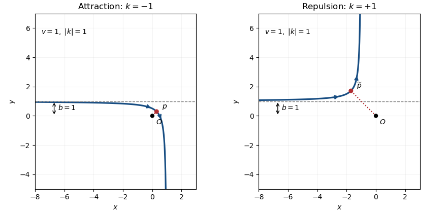
The hyperbola shown has a nonzero impact parameter. For $b=0$, the attractive radial orbit instead reaches the singular origin; there is no regular turning point with a finite closest-approach speed.

For nonzero $\omega$, the equilibrium points satisfy $\sin 2\theta =0$. The equilibrium point $\theta =0$ is stable: it puts the bead at the point farthest from the rotation axis. Writing $\theta =\eta$ small in the tangential ordinary differential equation givesThus the small oscillation is simple harmonic motion, with angular frequency $|\omega |$ and ordinary frequency $|\omega |/(2\pi )$.

The endpoints $\theta =\pm \pi /2$ represent the same rim point $O$. A perturbation there instead satisfies $\ddot{\eta }=+{\omega }^2\eta$ and is unstable. Equivalently, the centrifugal potential along the hoop is $-\frac{1}{2}{\omega }^2|\mathbf{r}{|}^2=-2a^2{\omega }^2{\cos }^2\theta$, whose minimum is at zero and maximum at $O$. If $\omega =0$, every bead position with zero relative velocity is an equilibrium point, but perturbing that velocity produces unrestored drift; there is no nonzero restoring frequency.

Because the contact is frictionless, the horizontal normal force is ${\mathbf{F}}_h=N\mathbf{n}$, with $N$ a signed outward component. Any vertical contact component balances Newtonian gravity and does not enter the horizontal equations. With $\mathbf{\omega }=\omega \hat{\mathbf{z}}$, the rotating reference frame equation givesSince $\hat{\mathbf{z}}\times \mathbf{\tau }=-\mathbf{n}$, $\mathbf{r}\cdot \mathbf{n}=2a{\cos }^2\theta$, and $\mathbf{r}\cdot \mathbf{\tau }=-a\sin 2\theta$, its normal and tangential components areHence the requested horizontal force vector isIts magnitude is the absolute value of the scalar coefficient. That coefficient need not always be negative: the constraint can exert either sign of normal force, depending on the bead's relative velocity. The tangential equation, which does not contain the reaction, is $\boxed{\ddot{\theta }=-({\omega }^2/2)\sin 2\theta }$.

Write the total remaining rocket mass as $\mathcal{M}=M+m(t)$, with $\dot{m}=-\alpha$. Over an interval $dt$, an exhaust mass $d{m}_e=\alpha dt$ is expelled backwards with inertial velocity $v-u$ to first order. Applying momentum conservation to the rocket and this exhaust givesCancellation and division by $dt$ give the rocket equationWith $M>0$, $m(t)=m_0-\alpha t$, and $0\le t\le m_0/\alpha$, integration givesAt burnout,The logarithm depends on the mass ratio, not on the burn rate. This follows from momentum conservation of the complete rocket–exhaust system; applying a constant-mass equation directly to the rocket alone would omit the momentum carried away.

For $0\le k<1$, the first burn reduces the total mass from $M+m_0$ to $M+(1-k)m_0$. The rocket equation therefore givesDetachment exerts negligible impulse, so the surviving second stage keeps velocity $v_1$. Its initial and final masses are $(1-k)(M+m_0)$ and $(1-k)M$, respectively. A second application of the rocket equation givesFor the single-stage comparison from rest, $v_{\mathrm{single}}=u\log (1+m_0/M)$. HenceEquality holds at $k=0$; for positive fuel and exhaust speed it is strict when $0<k<1$. This two-stage rocket with proportional fuel and body masses gains speed by discarding inert body mass before the last burn.

As $k\to 1^{-}$ the expression tends to $2u\log (1+m_0/M)$, but the surviving second-stage mass also tends to zero. At exactly $k=1$ there is no second stage, so its final speed is undefined and that limiting formula cannot be assigned to it. The first stage alone reaches the single-stage burnout speed before detachment. If $m_0=0$, neither design gains speed.

Assume the particle masses $m_i$ are fixed and their total mass $M={\sum }_i{m}_i$ is positive. The centre of mass and the relative position vectors areTheir weighted sum is zero, so differentiation gives ${\sum }_i{m}_i{\dot{\mathbf{y}}}_i=0$. Expanding the kinetic energy with ${\dot{\mathbf{x}}}_i=\dot{\mathbf{R}}+{\dot{\mathbf{y}}}_i$ makes the mixed term vanish:This kinetic-energy decomposition about the centre of mass separates translation from internal motion without assuming any particular force law.

For the rigid body, its relative velocity is ${\dot{\mathbf{y}}}_i=\omega \mathbf{n}\times {\mathbf{y}}_i$. The cross product identity for a unit vector gives $|\mathbf{n}\times {\mathbf{y}}_i{|}^2=|{\mathbf{y}}_i{|}^2-(\mathbf{n}\cdot {\mathbf{y}}_i{)}^2$, the squared perpendicular distance to the rotation axis. Hence the moment of inertia of the particle is $I_i=m_i[|{\mathbf{y}}_i{|}^2-(\mathbf{n}\cdot {\mathbf{y}}_i{)}^2]$, and summing the rotational kinetic energy yields

The dimensions are $[m]=\mathsf{M}$, $[\alpha ]=\mathsf{M}{\mathsf{T}}^{-1}$, $[u_0]=\mathsf{L}{\mathsf{T}}^{-1}$, and $[g]=\mathsf{L}{\mathsf{T}}^{-2}$. Under the stated model, $m,\alpha ,u_0,g$ are the only parameters determining the ascent time. If $m^p{\alpha }^q{u}_0^r{g}^s$ is dimensionless, then $p+q=0$, $r+s=0$, and $-q-r-2s=0$, leaving one independent dimensionless variable. One convenient choice isThus dimensional analysis fixes the form, but Newton's second law must determine the function $f$.

Take upward velocity as positive. Throughout ascent, Newton's second law with linear drag gives $m\dot{v}=-mg-\alpha v$. An integrating factor or direct solution of this linear ordinary differential equation givesThe first zero of this velocity is the highest point, soThis vertical ascent under linear drag has $T<u_0/g$ for $u_0>0$, since $\log (1+\lambda )<\lambda$. The limit $\alpha \to 0$ recovers the no-drag ascent time $u_0/g$; $u_0=0$ gives $T=0$.

Use a local orthonormal tetrad and units in which the speed of light is one. A particle has four-momentum $p^{\hat{a}}=E(1,\mathbf{e})$ and moves with velocity $\mathbf{e}$. Thus its energy density contributes $E$, its momentum density contributes $E{e}^i$, and its momentum flux contributes $E{e}^i{e}^j$. Integrating the phase-space distribution function gives the kinetic stress-energy tensor. The measure $d^{3}p/E$ is the future mass-shell Lorentz-invariant phase-space measure, so the same expression transforms as a spacetime stress-energy tensor; fixed state-counting or polarization factors are understood to be included in $f$.

Define $⟨F{⟩}_{\Omega }=(4\pi {)}^{-1}\int Fd\Omega$. The photon momentum measure is $d^{3}p=E^{2}dEd\Omega$, so every component of the kinetic stress-energy tensor has a radial factor $E^{3}dE=a^{-4}{ϵ}^{3}dϵ$. An isotropic background has $⟨e^i{⟩}_{\Omega }=0$ and $⟨e^i{e}^j{⟩}_{\Omega }={\delta }^{ij}/3$. HenceThis radiation pressure equation of state requires isotropy and masslessness, not a thermal spectrum.

The distribution perturbation is $\delta f=-ϵ{\bar{f}}^{\prime }(ϵ)\Theta$. Assume finite energy density and endpoint behavior ${ϵ}^4\bar{f}(ϵ)\to 0$ at zero and infinity, as for the Planck photon distribution. Integration by parts then givesConsequently the perturbed energy density and momentum density areSince $q^i=(\bar{\rho }+\bar{P})v^i=(4\bar{\rho }/3)v^i$, the photon angular temperature moments give $\delta =4⟨\Theta {⟩}_{\Omega }$ and $v^i=3⟨\Theta e^i{⟩}_{\Omega }$.

The sign of anisotropic stress must be specified. Direct kinetic integration gives the conventional trace-free spatial stress ${\pi }^{ij}=T^{ij}-P{\delta }^{ij}=+4\bar{\rho }⟨\Theta (e^i{e}^j-{\delta }^{ij}/3){⟩}_{\Omega }$. The PDF uses the opposite sign, ${\Pi }^{ij}=-{\pi }^{ij}$, equivalently $T^{ij}=P{\delta }^{ij}-{\Pi }^{ij}$. With that convention, all requested moments areTaking the spatial trace also givesThe angular temperature description assumes $\Theta$ is independent of photon energy; independent spectral distortions would require additional energy-dependent moments.

Let the constant mass density be $\rho >0$ and put ${\mathbf{v}}_a=\mathbf{B}/\sqrt{{\mu }_0\rho }$, the Alfvén velocity. Since both the velocity and the magnetic field have zero divergence, the magnetic tension and magnetic pressure decomposition of the Lorentz force givesThe Newtonian gravitational potential $\Phi$ remains in $\psi$; uniform mass density does not justify dropping a prescribed gravitational acceleration. Adding and subtracting the two equations proves the Elsässer variable equationsHere ${\mathbf{z}}^{\pm }=\mathbf{u}\pm {\mathbf{v}}_a$; each Elsässer variable is transported by the other.

Define $I_{\pm }={\int }_V|{\mathbf{z}}^{\pm }{|}^{2}dV$. Taking the dot product with $2{\mathbf{z}}^{\pm }$ gives the Elsässer energy invariant balanceThe divergence theorem proves $d{I}_{\pm }/dt=0$ whenever the net boundary flux vanishes. In particular, $\mathbf{u}\cdot \mathbf{n}=\mathbf{B}\cdot \mathbf{n}=0$ makes ${\mathbf{z}}^{\pm }\cdot \mathbf{n}=0$, so both fluxes vanish pointwise. Periodic boundary conditions or decay at infinity are also sufficient. These boundary conditions matter: fixed volume alone gives no conservation.

The kinetic energy plus magnetic energy isExpanding $|\mathbf{u}\pm {\mathbf{v}}_a{|}^2$ and using the cross-helicity definition yieldsBoth energy and cross-helicity therefore follow from the two Elsässer energy invariants. The quantity $E$ here is exactly the requested kinetic energy plus magnetic energy, without an additional gravitational term.

Use $v=|u_r|>0$ for the radial speed and distinguish the central mass $M$ from the Mach number $\mathcal{M}=v/c$. In each smooth nonzero-flow region, mass conservation, the adiabatic equation of state, and the Bernoulli equation giveHere $K>0$ is constant on a smooth isentropic flow branch, $c$ is the adiabatic sound speed, and $\mathcal{E}$ is the Bernoulli function. Either sign of $u_r$ is possible. The positive-radius nondimensionalization in the question requires $\mathcal{E}>0$; flows with $\mathcal{E}\le 0$ do not have these positive $r_s,x,\lambda$ and require another scaling.

Indeed, the supplied adiabatic process equations give $D(p{\rho }^{-3/2})/Dt=0$, so $K$ is spatially constant along a steady nonzero radial fluid flow. The adiabatic sound speed is $c^2=(\partial p/\partial \rho {)}_s$, and the specific enthalpy is $h=c^2/(\gamma -1)=2c^2$. The radial Euler momentum equation, $vdv/dr=-{\rho }^{-1}dp/dr-GM/r^2$, integrates to $\mathcal{E}$ because $dh=dp/\rho$ on this isentropic flow branch.

Put $D=[j(3K/2{)}^2{]}^{2/5}$. Eliminating the mass density from the continuity equation givesWith $y={\mathcal{M}}^{2/5}$, the Bernoulli equation becomesTherefore the physical constants of the spherical polytropic flow with adiabatic exponent three halves are

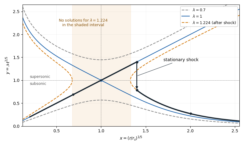
For $t>0$, $F^{\prime }(t)=4(t^5-1)/t^2$, so $F$ decreases from infinity to its unique minimum $F(1)=5$, then increases to infinity. This completely determines the algebraic curves. For $0<\lambda <1$, there are two disconnected branches at every $x>0$, one subsonic flow with $y<1$ and one supersonic flow with $y>1$. For $\lambda =1$, the line $y=x$ and a decreasing branch meet at $(1,1)$. Their slopes are $+1$ and $-1$, since the leading expansion is $F(1+\eta )=5+10{\eta }^2+O({\eta }^3)$. For $\lambda >1$, solutions exist only where $F(x)\ge 5\lambda$: if $x_{-}<1<x_{+}$ solve $F(x_{\pm })=5\lambda$, there is a forbidden interval $x_{-}<x<x_{+}$. At either endpoint the two branches turn at $y=1$ and have an infinite slope.

A smooth sonic point needs $F^{\prime }(x)=F^{\prime }(y)=0$; hence a regular sonic transition requires $\lambda =1$ and $r=r_s$. The critical speed of a polytropic flow is then $c_s^2=GM/(2r_s)=2\mathcal{E}$, and the allowed mass flux is $j=(2\mathcal{E}{)}^{5/2}{r}_s^2/(3K/2{)}^2$. Here the subscript on $c_s$ denotes evaluation at the sonic point, rather than the isothermal sound speed convention used in the next solution.

The simple transonic branch is $y=x$. Direct substitution givesThus the radial velocity has constant magnitude, while the mass density and pressure scale as $r^{-2}$ and $r^{-3}$. For an outward fluid flow, this is a subsonic flow becoming a supersonic flow as its adiabatic sound speed decreases.

On the other transonic branch, $y$ decreases as $x$ increases. At large $r$, the terms $4/y$ and $x^4$ dominate, giving $y\sim 4x^{-4}$. At small $r$, the terms $y^4$ and $4/x$ dominate, giving $y\sim 4^{1/4}{x}^{-1/4}$. The resulting asymptotic expansions areFor inward fluid flow, these are the nearly static reservoir at infinity and the inner free fall region of Bondi accretion. The specific enthalpy is smaller than $GM/r$ in the inner limit, which explains free fall. Reversing the radial velocity gives a decelerating outflow with the same profiles. The formal small-$r$ limit describes the point-mass model: if the spherical gravitating body has a finite surface, the exterior solution stops there.

A stationary, nonradiative normal shock wave conserves the mass flux and the sum $v^2/2+h$, while the Newtonian gravitational potential is continuous across its thin layer. Hence $\mathcal{E}$ and $r_s$ are unchanged. The entropy production in a perfect-gas shock increases $K=p/{\rho }^{3/2}$, soMore explicitly, the Rankine-Hugoniot condition for $\gamma =3/2$ gives, with upstream $m={\mathcal{M}}_1^2>1$,Thus the shock wave jumps vertically, at the same $x$, from the supersonic flow to a subsonic flow on a larger-$\lambda$ curve. The figure illustrates an outward flow on $y=x$ with a shock wave at $x=1.4$; the downstream subsonic flow has $\lambda \simeq 1.224$ and continues to larger $x$. The shock wave radius is an additional boundary-data choice, rather than being determined by the smooth equations alone.