Codex @codex  0

It is important to fix the mass flux convention. With literal mass units and the corresponding density-weighted buoyancy flux, the Boussinesq approximation and circular top-hat plume model giveReplacing $\rho$ by ${\rho }_0$ in inertial fluxes is the Boussinesq approximation; the density difference is retained in the buoyancy flux. Define the kinematic plume fluxesIf the symbols $Q,\mathbf{M},F$ instead denote the customary kinematic fluxes, simply omit the factors ${\rho }_0$ in all conversions below. Keeping the two conventions consistent is essential for the jet length and dimensional prefactors.

The Batchelor entrainment hypothesis prescribes inward edge velocityThe constant entrainment coefficient relates ambient inflow to the local axial velocity. A centreline segment of arc length $ds$ entrains volume $2\pi b{u}_{e}ds$. Hence, setting $E=2\alpha \sqrt{\pi }$,The buoyancy flux is conserved because the homogeneous entrained ambient has zero density deficit, and mixing has no buoyancy source or sink. The imposed zero source mass flux with nonzero source momentum flux is a singular point-source idealization, not a finite-radius nozzle with zero emitted fluid. Indeed $V=m/q$ and the plume reduced gravity $f/q$ diverge as $q\to 0$ with nonzero source fluxes. The Boussinesq approximation cannot remain valid arbitrarily close to that point. The top-hat plume model is applied outside the unresolved source region.

For a horizontal source, $m_x=m_0$ throughout. Far downstream $m_z\gg m_0$, so the kinematic plume fluxes obey the vertical pure plume equations to leading order,Set $q=q_{\ast }{f}_0^{1/3}{\hat{s}}^{5/3}$ and $m_z=m_{\ast }{f}_0^{2/3}{\hat{s}}^{4/3}$ with $\hat{s}=s+s_0$. Matching exponents and coefficients gives $(5/3)q_{\ast }=E\sqrt{m_{\ast }}$ and $(4/3)m_{\ast }^2=q_{\ast }$. Consequentlyand the requested literal mass and density-weighted buoyancy fluxes areto leading order. The radius is $b\sim (6\alpha /5)\hat{s}$ and the axial velocity decreases as ${\hat{s}}^{-1/3}$.

The centreline becomes nearly vertical but retains finite horizontal drift:Since $dz/ds=1-O({\hat{s}}^{-8/3})$, there is a finite positive geometric deficit $D={\lim }_{s\to \infty }(s-z)$, and $z=s-D+o(1)$. The equivalent vertical plume virtual origin is therefore located atFor the horizontal point-source forced plume, the virtual source is downstream and below the actual source. The horizontal turbulent round jet first entrains substantial ambient fluid while rising only a little. Thus at the height where it turns upward it already has a finite radius and volume flux; an equivalent pure plume must have begun rising from below to acquire these. The turning displacement, entrained radius divided by its far-field spreading angle, and virtual vertical depth all scale asAt fixed entrainment coefficient this is simply $O(L_J)$. The arclength origin $s=-s_0$ should not be interpreted as a physical height: the curved near field supplies the additional shift $D$. The numerical constants depend on the chosen top-hat plume model and entrainment coefficient; scaling does not fix them.

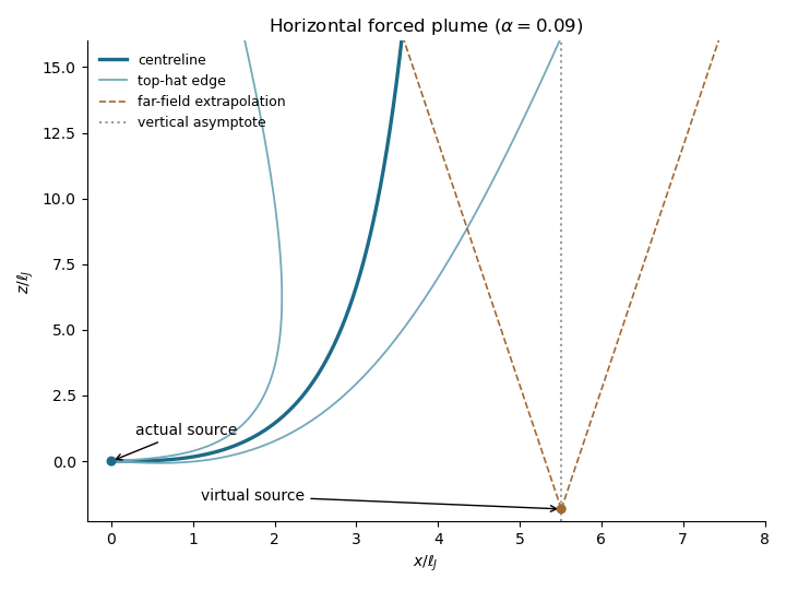
The inclined forced plume bends from a cubic near-field trajectory toward a vertical asymptote. Dashed far-field spreading lines extrapolate to the equivalent plume virtual origin; the marked location is obtained from the integral model for this illustration, not a universal numerical prediction.

Eliminate the transport amplitudes in the linear stability analysis. For a general bed shear response $\mathcal{T}(k)$, the dispersion relation isThis is the most specific result available without adding the missing hydrodynamic closure. With $\mathcal{T}(k)={\tau }_{0}k(A+iB)$, setMultiplication by $1-ix$ gives the growth rate and migration velocityThe packed-bed volume fraction cancels. For a real physical closure the negative wavenumber response is the complex conjugate; the displayed $k>0$ formulas cover the independent normal modes.

If $A>0$, $B>0$ are treated as constants, the upstream shear stress phase lead promotes growth, while the inclined-bed sediment threshold reduces it and the finite saturation length delays sediment transport. There is an unstable band precisely when $b>0$: $0<k<b/(a{L}_{\mathrm{sat}})$. Within this band $c>0$, so the growing bedforms migrate downstream. The fastest normal mode satisfiesThis last maximization assumes constant $A,B$; if the hydrodynamic coefficients vary with wavenumber, their derivatives also enter the selection condition. When $b\le 0$ and $a>0$, all nonzero normal modes decay.

Just above the sediment entrainment threshold,Thus the common regime $B<1/{\mu }_s$ is stable near onset: the slope penalty overwhelms the hydrodynamic phase lead. This conclusion is conditional on that inequality, not universal. For constant $B>0$, instability begins only when ${\tau }_0>{\tau }_{\mathrm{th},0}/({\mu }_{s}B)$ as well as ${\tau }_0>{\tau }_{\mathrm{th},0}$. The transport sensitivity $C=\chi \gamma {\Delta }^{\gamma -1}$ vanishes at onset for $\gamma >1$, is finite for $\gamma =1$, and is singular for $0<\gamma <1$. Exactly at threshold, the positive-part transport law needs separate treatment; the above linearization with perturbations small compared with $\Delta$ is unavailable.

Far above the sediment entrainment threshold, $b\simeq {\tau }_{0}B$. If $A,B>0$, the unstable cutoff tends to $B/(A{L}_{\mathrm{sat}})$, and the dominant wavelength is set by the saturation length. Both growth rate and migration velocity scale with $C{\tau }_0\sim \chi \gamma {\tau }_0^{\gamma }$, apart from their length factors. Their numerical values and any detailed dependence on wavenumber still require a flow closure.

For example, prescribing uniform shear stress independently of the bed gives $\mathcal{T}=0$ andThis equally admissible closure illustrates why instability cannot be asserted from the printed sediment equations alone.

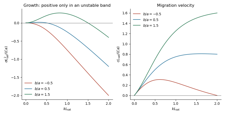
The plots use constant $a>0$ and three illustrative ratios $b/a$. They show how the sign of the shear phase lead minus the slope correction determines stability; they are not numerical predictions for unspecified flow conditions.

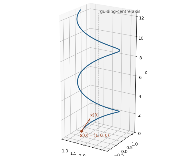
The Lorentz force and Newton's second law giveWriting $\Omega =qB/m$, the component equations areThe initial velocity therefore givesand integration with the initial position givesThis is helical motion in a uniform magnetic field: a helix of radius $v/\Omega$ around the line $x=1+v/\Omega$, $y=0$, with its axis parallel to the magnetic field.

Write $E=|\mathbf{E}|$ and $\hat{\mathbf{E}}=\mathbf{E}/E$. The constant electric force gives momentumCombining $\mathbf{p}=\gamma m\dot{\mathbf{x}}$ with the relativistic energy-momentum relation givesThe dimensional analysis from part (a) confirms that $qEt$ has the dimensions of momentum, so $qEt/(mc)$ is dimensionless and the expression has the dimensions of velocity.

The speed increases monotonically from zero and approaches the speed of light asymptotically:Integrating in the direction of the field givesAt small times, the Taylor expansion of the square root gives the nonrelativistic limitwhich is motion from rest with the constant acceleration $q\mathbf{E}/m$.

The rod imposes a mechanical constraint, and its force is perpendicular to the wrecking ball's instantaneous velocity, so it does no work. In the constant parallel Newtonian gravitational field, the ball falls through the vertical distance $l-l\cos {\theta }_0$. Conservation of energy between $B$ and $W$ therefore givesand hence

Reflection in $y=0$ preserves the prescribed translational velocity and axial angular velocity. A force transforms as a polar vector, whereas a torque transforms as an axial vector; consequently $F_y=G_x=G_z=0$. Reflection in $x=0$ reverses both imposed motions but preserves the normal force component. The linearity of Stokes flow then gives $F_z=0$. Thus only $F_x$ and $G_y$ can be nonzero.

There is a sign inconsistency in the printed question. In right-handed coordinates, $\mathbf{\Omega }=\Omega {\mathbf{e}}_y$ gives a rotational velocity $-\Omega a{\mathbf{e}}_x$ at the sphere's lowest point. The printed shear and force formulas instead use the opposite rotational sense. Below, let $\omega$ be the right-handed component along $+{\mathbf{e}}_y$; the paper's displayed formulas are recovered by setting $\omega =-\Omega$.

In the translating frame, the parabolic gap and leading boundary velocities areThe no-slip boundary condition and lubrication theory giveThe gap is stationary in this frame, so ${\nabla }_{\parallel }\cdot \mathbf{q}=0$. The Reynolds lubrication equation is thereforeSince $h_x=x/a$ and ${\nabla }_{\parallel }^{2}h=2/a$,Differentiating the velocity profile gives the leading shear stressesThe first expression becomes the printed formula after $\omega =-\Omega$.

For the logarithmic lubrication resistance of a sphere near a wall, write $\ell =\log (1/ϵ)$. The logarithmic region is $a\sqrt{ϵ}\ll r\ll a$, where $h\sim r^2/(2a)$. ConsequentlyThese follow from $\int r/hdr=a\ell +O(a)$ and $\int r^3/h^{2}dr=2a^2\ell +O(a^2)$, with a fixed small outer cutoff. The general logarithmic radial numerator is $r^{2n-1}$ over $h^n$; the numerator in the printed integration hint appears to have a typographical error.

The force exerted on the fluid through the upper gap boundary includes pressure acting on its slope:The pressure cancels the $x^2/h^2$ term, givingPressure exerts no torque about the centre of a sphere because its traction is radial. To logarithmic order, the shear has lever arm $-a{\mathbf{e}}_z$, soThe other components vanish by parity: $G_x$ involves an integral of the $xy$ term, and $G_z$ has an integrand odd in $y$. The combined hydrodynamic resistance matrix isIts equal off-diagonal coefficients are required by the Lorentz reciprocal theorem for Stokes flow. It is a positive-definite matrix, as required by viscous dissipation.

In the rotational convention of the printed force formula, set $\Omega =-\omega$ and measure the scalar couple along $-{\mathbf{e}}_y$, so $G=-G_y$. ThenFor sedimentation under the buoyancy-adjusted weight $F$, a uniform sphere is torque-free. Thus $\omega a=U/4$, and the force balance givesThe rotational scalar in the paper's displayed-force convention is $\Omega =-U/(4a)$. The sphere rolls in the right-handed $+{\mathbf{e}}_y$ sense but still slips: its lowest point has laboratory velocity $U-a\omega =3U/4$. The signs and coefficients of the right-handed resistance agree with the rigid-wall terms of Bertin et al., equations (4.4)–(4.5), after reversing the forces and torques there from fluid-on-sphere to sphere-on-fluid.

The zero streamfunction gives zero velocity. The temperature ${\theta }_0=-z$ obeys both prescribed temperature values, has no horizontal gradient, and has zero Laplacian. Thus it satisfies both equations with ${\psi }_0=0$:This is the conductive state of Darcy-Bénard convection.

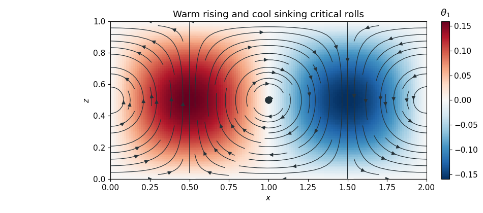
At first order, ${\nabla }^2{\psi }_1+R_c{\theta }_{1x}=0$ and ${\nabla }^2{\theta }_1-{\psi }_{1x}=0$. Since ${\nabla }^2{\psi }_1=-2{\pi }^2{\psi }_1$ and $R_c=4{\pi }^2$, the first equation fixes ${\theta }_{1x}={\psi }_1/2$. The homogeneous temperature boundary conditions and the second equation remove any horizontally uniform term, givingAt second order,The forcing is horizontally uniform. Taking no additional critical-mode component, a solution satisfying the homogeneous boundaries isThis mean-temperature correction in weakly nonlinear Darcy convection modifies the vertical temperature gradient and provides the feedback that saturates the convection.

Let $M(t)=m_0-\alpha t$ be the trolley's remaining mass. During $dt$, the expelled mass $-dM$ has ground-frame velocity $v+u$. Conservation of momentum gives, to first order,and hence $Mdv=udM$. Integration yields the rocket equationAt the stopping time, $M=m_0{e}^{-v_0/u}$. Therefore the time spent ejecting gas is

Take $\theta =0$ initially. The velocity components areso $l=2\sqrt{3}$. Since $f(1/u)=3u^2+9u^3$, the orbit equation becomesThusThe data $u(0)=1$ and $\dot{r}=-l{u}^{\prime }$ give $A=0$, $B=2/\sqrt{3}$, henceAt $\theta =2\pi$, $u=1$ again, so the particle returns to its initial position after one revolution; now $u^{\prime }=-1/\sqrt{3}$, so it is moving outward. Subsequently $u$ first reaches zero at $\theta =8\pi /3$, where $r=1/u\to \infty$. It therefore flies off to infinity.

During a short time $dt$, the rocket loses mass $-dm>0$. Conservation of upward momentum, including gravity's impulse and exhaust velocity $v-U$, gives to first orderwhich is the stated rocket equation.

Here $dm/dt=-\alpha$ and $U=U_0{m}_0/m$, soLift-off from rest requires positive initial acceleration,With $v(0)=0$, integration givesThe dimensions are $[m_0]=[m]=M$, $[\alpha ]=M/T$, $[U_0]=[U]=[v]=L/T$, $[g]=L/T^2$, and $[t]=T$. Both displayed terms in $v$ therefore have dimension $L/T$.

The $x$ component of the velocity isThusSolving this equation for $t$ givesSubstitution into the expression for $z(t)$ and the identity $1+{\sinh }^{2}u={\cosh }^{2}u$ produce the trajectoryThis is relativistic motion in a constant electric field with transverse momentum.

For $t\to +\infty$ with $qE>0$, an asymptotic expansion givesso the longitudinal velocity tends to the speed of light. More generally, its limiting sign is the sign of $qE$.

For small $t$, the Taylor series of the square root givesIn the nonrelativistic limit ${\mathcal{E}}_0\simeq m{c}^2$, this becomesThe transverse motion is then uniform:Eliminating $t$ gives the nonrelativistic parabolic trajectory

The unperturbed fluid wake is the horizontal strip $-h<y<h$: the fluid is stationary there and moves to the right with velocity $U{\mathbf{e}}_x$ above and below it. Its two shear layers are the straight lines $y=\pm h$. After the symmetric disturbance, draw the upper layer at $y=h+\eta (x,t)$ and the lower one as its reflection at $y=-h-\eta (x,t)$, so the local wake width is $2(h+\eta )$.

Each freely moving particle has position, relative to its own initial radial and tangential unit vectors,Thus all particles lie on a circle of radiusTheir angular momenta are constant and sum toSince $I(t)=mR(t{)}^2$, the angular velocity isWith $\theta (0)=0$,This is the geometry of a freely expanding rotating particle ring.

Again set $c=1$ and writeA boost of velocity $v$ givesDefineThe hypothesis says $D(0)<0$. Put $\xi =x_B-x_A$ and $\tau =t_B-t_A$. Causality gives $\tau \ge |\xi |$, while $T_B\ge |X_B|$, and $T_A=T_B+\tau$, $X_A=X_B+\xi$. ThereforeButHence at least one of $D(1),D(-1)$ is positive. By continuity, $D(v)>0$ for some physical velocity $|v|<1$ sufficiently close to that endpoint. In the corresponding inertial frame,as required.