Codex @codex  0

For a two-dimensional internal gravity wave with fixed horizontal wave number $k\ne 0$, the vertical velocity amplitude satisfiesThis follows from the Linearized Boussinesq equations just as in part (a), allowing the background buoyancy frequency to vary. The WKB approximation gives locallyIt requires slowly varying stratification compared with the local vertical wavelength, in particular $|m_z|\ll m^2$, and a small-amplitude wave in the inviscid, nonrotating regime. Propagation requires $N>|\omega |$; where $N<|\omega |$, the local vertical wave number is imaginary and the solution is evanescent. Turning levels and abrupt changes need a separate connection calculation. Finite viscosity, background flow, rotation or nonlinear effects require modifications of this model.

The ray tracing equations use the local dispersion relation as a Hamiltonian:The stationary, horizontally uniform background conserves the frequency and horizontal wave number. In two dimensions the group velocity gives $dx/dz=-m/k$. For the specified buoyancy frequency and $\omega =1$, $m^2=256k^2{z}^2$. Hence for $z>0$ the two geometric internal-wave rays through the specified point areEach curve has both directed propagation senses, giving four local directed rays. Their formal intersections with $z=0$ are $x=-8$ and $x=8$.

At $z=0$, $N=\omega$ and $m=0$: this is a double-zero internal-wave turning level, since $m^2$ touches zero without changing sign. The ray becomes vertical geometrically, but its group velocity tends to zero. Taking $k>0$ without loss of generality, the downward branch hasThe formal travel time diverges logarithmically as $z\to 0$. Meanwhile $|m_z|/m^2=1/(16|k|z^2)$ grows, so the WKB approximation fails before that limit; its predicted $|m{|}^{-1/2}$ amplitude cannot be extrapolated to infinity. The spatial ray reaches a finite limiting position, but finite-wavelength behaviour near the zero must be found beyond WKB. There is no evanescent half-space supplied by this particular $N(z)$, so ordinary simple-turning-point reflection cannot be assumed solely from the local ray construction.

The Boussinesq approximation requires $\delta =(\rho -{\rho }_0)/{\rho }_0=\varphi ({\rho }_p/{\rho }_0-1)\ll 1$. The reference mass density ${\rho }_0$ can then be used in inertia, while the small density excess is retained in buoyancy. Dilute particle volume fraction $\varphi \ll 1$ alone does not suffice if ${\rho }_p/{\rho }_0$ is exceptionally large. Define $G=g({\rho }_p-{\rho }_0)/{\rho }_0$, so the reduced gravity is $g^{\prime }=G\varphi$.

The shallow water equations require depth small compared with the horizontal evolution scale, weak vertical acceleration and approximately hydrostatic pressure. Here the ambient is deep and quiescent, so its leading contribution is a hydrostatic reference pressure; the excess pressure in the layer is ${\rho }_{0}G\varphi (h-z)$. The model also needs nearly uniform streamwise velocity across the section and the stated absence of secondary circulation. The advancing gravity current nose is a separate region where these assumptions can fail.

A nearly uniform particle volume fraction can be maintained by turbulent mixing with eddy diffusivity $K_z$, provided $h^2/K_z\ll h/w$ and the mixing time is short compared with horizontal advection and bulk evolution. Equivalently, $wh/K_z\ll 1$ keeps the bulk settling-induced gradient small. The particles should respond rapidly enough to follow the mixing motions. A thin boundary layer adjacent to the absorbing bed or walls need not be well mixed.

Uniform bulk concentration does not imply zero sedimentation. The relative downward particle velocity still supplies a particle deposition flux of approximately $w\varphi$ to an absorbing boundary. Mixing redistributes the remaining particles and maintains the bulk concentration profile while its overall level decreases; it need not suspend every particle indefinitely. Deposition requires negligible resuspension in the model.

At the gravity current nose, the depth and velocity change over a distance comparable with the depth, with appreciable vertical acceleration and mixing. The hydrostatic approximation and the depth-uniform interior model do not resolve that structure. A suitable gravity-current front condition iswith a positive, order-one Froude number determined by the nose closure and geometry. It is not fixed by the interior equations alone. This definition uses $\sqrt{g^{\prime }h}$; if the front condition is expressed using $c=\sqrt{g^{\prime }h/2}$, its numerical coefficient changes by $\sqrt{2}$.

For a late-time gravity-current box model, take the depth and particle volume fraction to be uniform over $0<x<X(t)$, and neglect entrainment and resuspension. The initial volume is $\mathcal{V}=\beta h_0^{2}L/2$, soThe total particle volume is $\mathcal{V}\varphi$. Deposition over the projected boundary width gives $d(\mathcal{V}\varphi )/dt=-\beta hXw\varphi$. With the specified hindered settling factor, the prismatic triangular-channel gravity-current box model isInitializing this approximate model with $X(0)=L$ and $\varphi (0)={\varphi }_0$ matches the original volume and concentration; it does not assert that the immediate dam-break flow is a uniform box.

Eliminate time to obtainSince the left primitive is $2\mathrm{artanh}\sqrt{\varphi }$, the hindered-settling runout invariant in a prismatic triangular channel isThis relation, the volume constraint and $\dot{X}$ determine the late-time evolution. If desired, the time is given by the quadrature $t={\int }_L^{X(t)}[\mathrm{Fr}\sqrt{G\varphi (s)h_0\sqrt{L/s}}{]}^{-1}ds$. The physical branch has nonnegative right-hand side in the boxed relation; it ends when that expression reaches zero.

Thus the limiting runout length of a gravity current, measured from the closed end, isThe advance beyond the dam is $X_{\infty }-L$. In the dilute limit, $\mathrm{artanh}\sqrt{{\varphi }_0}\simeq \sqrt{{\varphi }_0}$. The ideal model approaches its finite runout length of a gravity current only as $t\to \infty$: near the limit $\varphi$ decays exponentially with rate $2w_0/h_{\infty }$ and the front speed tends to zero. The exponent $7/4$ uses the prismatic triangular geometry; a channel widening with $x$ has a different volume constraint and runout law.

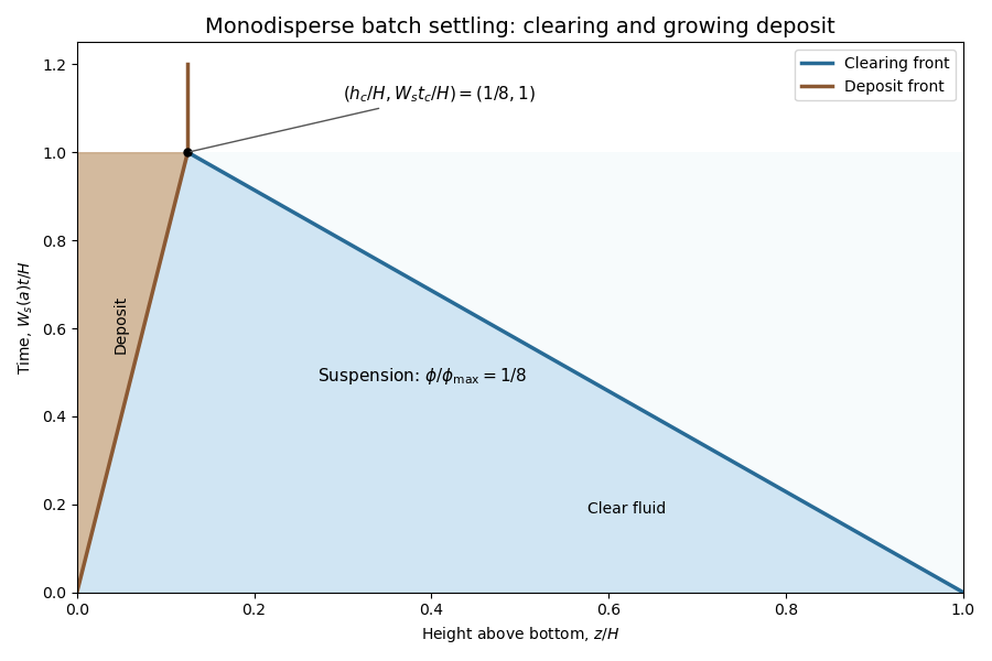
Use downward distance $y=H-z$, with $z$ the height above the bottom, and write $W=W_s(a)>0$. This convention will also reproduce the printed negative deposit-front velocity in part (d). The ideal simple-cubic sphere packing has packing fraction $\pi /6$; leaving ${\varphi }_{\max }$ symbolic keeps the jump calculation independent of its value. In suspension, the kinematic sedimentation equation isIntegrate this conservation law across a moving discontinuity to obtain the Rankine-Hugoniot conditionThe brackets denote values on the increasing-$y$ side minus those on the other side. A sedimentation shock is a concentration jump moving at this secant slope of the particle flux. Deposited material is stationary and has zero flux.

For the upper clearing front, the states are $0$ and ${\varphi }_{\max }/8$, giving $U_1=7W/8$ downward. For the lower deposition front, the states are ${\varphi }_{\max }/8$ and ${\varphi }_{\max }$, giving $U_2=-W/8$, upward. ThusIn terms of height above the bottom, the shock paths areThey meet when $H=Wt$. Therefore complete settling occurs atThe final height also follows directly from particle volume fraction conservation, ${\varphi }_{\max }{h}_c=({\varphi }_{\max }/8)H$. The stationary deposit after the meeting carries no particle flux.

The diagram plots time vertically against height, as requested. Its shock slopes have the opposite spatial sign to $U_1,U_2$, because those velocities were defined in the downward coordinate.

At a fixed height, first determine the stored quantities per unit vertical height and per unit length along the line source. With $\Delta \rho =\rho -{\rho }_0$, the triangular-profile line plume has the useful profile integralThe geometric volume is $\mathcal{A}=2b$; the mass is $\mathcal{D}={\rho }_0{I}_0+\Delta \rho I_1=b(\rho +{\rho }_0)$. The upward momentum is $\mathcal{P}=W({\rho }_0{I}_1+\Delta \rho I_2)$, while the buoyancy force is $\mathcal{B}=-g\Delta \rho I_1$. ThusHere positive buoyancy corresponds to a rising light plume. If instead buoyancy is defined kinematically, divide $\mathcal{B}$ by ${\rho }_0$; the density-weighted convention here is the one matching the printed equations.

Multiply each local density by the vertical velocity to obtain the fluxes through a horizontal section, still per unit source length:In particular, the stored momentum equals the mass flux $Q$, and the buoyancy flux is $F=g({\rho }_{0}V-Q)$. The different triangular-profile factors in storage and flux must not be replaced by top-hat coefficients.

The Batchelor entrainment hypothesis models turbulent ingestion of ambient fluid through the plume edges. A self-similar turbulent plume has a spreading rate proportional to its axial velocity scale; the hypothesis represents the unresolved mixing by an inward edge speed proportional to that scale. For the prescribed centreline velocity, the Boussinesq approximation givesThe entrainment coefficient $\alpha$ is dimensionless and depends on the chosen velocity/profile convention and mixing regime. Here $e$ is the inward entrainment speed relative to the moving plume boundary, and the factor two counts its two sides.

A suitable density-corrected extension is $e=\alpha W\sqrt{\rho /{\rho }_0}$, representing the reduction in ambient ingestion for a much lighter non-Boussinesq plume. It reduces to the boxed closure when $|\rho -{\rho }_0|\ll {\rho }_0$. This is a phenomenological model, not an exact identity for arbitrary turbulent flow. Woods's non-Boussinesq plume model uses this density correction. The balances in part (c) can be written with either closure before taking their common Boussinesq limit.

Choose $x=0$ at the contact line, with $x>0$ pointing into the mountains and the plate moving in the positive $x$ direction at speed $U>0$. Let $z=0$ be the plate. For viscous mountain spreading over an underthrust plate, the lubrication approximation assumes slow horizontal variation, hydrostatic pressure $p=\rho g(h-z)$, and $\mu u_{zz}=p_x=\rho g{h}_x\equiv G$. Impose no slip at the plate and zero tangential traction at the free surface. Without sediment,The horizontal mass flux is $\rho q$. For a steady mountain range with no mountain material entering across its contact line, $q=0$. Therefore $h_x=3\mu U/(\rho g{h}^2)$, and the vanishing height at the bare contact gives the mountain profileThe large slope extremely close to $x=0$ is an inner region where the lubrication approximation ceases to be quantitatively valid.

Now let sediment occupy $0<z<d$ and mountains $d<z<h$, with $H=h-d$ the mountain-material thickness and $M={\mu }_s/\mu$. Equal densities make $G=\rho g{h}_x$ the same in both layers. Continuity of velocity and shear stress at $z=d$, no slip at $z=0$ and zero shear at $z=h$ give the shear stress $G(z-h)$ throughout. Thus the two velocity profiles areTheir volume fluxes areMultiplying by $\rho$ gives the separate mass fluxes. The coupled conservation of mass equations areThis is the sediment-lubricated viscous mountain model. It includes shear-driven transport by the plate and pressure-driven gravitational spreading.

In steady state the mountain-material flux is zero, while the upstream uniform sediment layer has $q_s=U{d}_{\infty }$. For $H>0$ this givesEliminating $G$ proves the algebraic thickness relation:At the contact $H\to 0^{+}$, the last coefficient must vanish. The nonzero physical solution is consequentlyThe condition comes from the limiting zero flux per unit mountain thickness, not merely the automatic vanishing of $q_m$ at $H=0$. The surface slope anywhere under the mountains isLower sediment viscosity flattens the near-contact surface, while its contact height remains $3d_{\infty }$. Far inside, where $H\gg d/M$, the mountains recover the bare-layer slope scaling. The formulas determine the mountain profile by the algebraic relation plus this first-order equation. For example, put $\delta =d/d_{\infty }$ and $w=H/d$; the physical root satisfies $2M(\delta -1)w^2+3(\delta -2)w+\delta -3=0$, taking $w\ge 0$ for $1<\delta \le 3$. This selects the branch smoothly connected to the contact.

In front of the contact, $x<0$, there is only sediment, so $h=d$ andDefine $\ell =\rho g{d}_{\infty }^3/(3{\mu }_{s}U)$ and $P(\delta )={\delta }^3/3+{\delta }^2/2+\delta +\ln (\delta -1)$. Integrating from the contact yields the upstream basin profile of a sediment-lubricated mountain:Equivalently, $d(x)=d_{\infty }{P}^{-1}(P(3)+x/\ell )$ on $1<\delta \le 3$. The inverse is uniquely defined because $P^{\prime }(\delta )={\delta }^3/(\delta -1)>0$; an elementary explicit inverse is unnecessary. This profile tends to $d_{\infty }$ as $x\to -\infty$, approaches $3d_{\infty }$ at the contact and has the same surface slope there as the mountain branch. Its far-field excess decays exponentially on length scale $\ell$, which increases as the sediment viscosity decreases.

The canonical momenta are $p_x=m\dot{x}$, $p_y=m\dot{y}+qBx$, $p_z=m\dot{z}$. The Legendre transform in mechanics givesHamilton's equations areThus $\ddot{x}=\Omega \dot{y}$, $\ddot{y}=-\Omega \dot{x}-qE/m$, and $\ddot{z}=0$, where $\Omega =qB/m$. The signs also follow from $\mathbf{E}=-E{\mathbf{e}}_y$ and $\mathbf{B}=B{\mathbf{e}}_z$.

For $Bq\ne 0$, put $v_d=-E/B$, $a=v_{x0}-v_d$, $b=v_{y0}$. The motion isDifferentiation verifies both equations and all initial conditions. The centre of the circular motion has the electric drift velocity $-E{\mathbf{e}}_x/B$. For $B=0$, take $x=x_0+v_{x0}t$, $y=y_0+v_{y0}t-qE{t}^2/(2m)$ and the same $z$. For $q=0$, the particle moves freely.

In the laboratory frame the lower wall has velocity zero and the cylinder surface has velocity $U$. Solving $\mu u_{yy}=p_X$ with these no-slip conditions givesThe relative velocity in the cylinder frame is $u-U$. Its flux is constant by incompressibility:Equal pressures at the two infinities require $\int p_{X}dX=0$. Put $I_j=\int h^{-j}dX$; then $q=-(U/2)I_2/I_3$. With $X=\ell s$ and $h=h_0(1+s^2)$, the given integrals yield $I_2/I_3=4h_0/3$. Hence $q=-2U{h}_0/3$ andIndeed $p=2\mu UX/h^2$ has this derivative and tends to ambient pressure at both ends. The distinction between the constant comoving flux and the varying laboratory flux is necessary because the gap translates.

Reflection about the closest point leaves the gap geometry unchanged and reverses the direction of translation. The linear Stokes equations make the excess pressure change sign when the imposed velocity changes sign. Combining reflection with this linearity shows that pressure is odd in $X$. Its leading normal force on the stationary plane therefore cancels between the two sides, giving ${\mathbf{e}}_y\cdot \mathbf{F}=0$ in the lubrication limit. Normal viscous stresses are of smaller order in the aspect ratio. This uses symmetry only, rather than a pressure calculation.

Use an Earth-centred rotating reference frame, with Earth's constant angular velocity vector $\mathbf{\omega }$. The vectors $\mathbf{r}$, $\mathbf{v}$, and $\mathbf{a}$ are the particle's position, velocity, and acceleration measured in that rotating frame. The vector $\mathbf{g}$ is the gravitational acceleration due to the actual gravitational force, expressed in the same axes; it excludes the separate centrifugal acceleration. The remaining term $-2\mathbf{\omega }\times \mathbf{v}$ is the Coriolis acceleration. A constant rotation axis and an unaccelerated Earth-centred origin account for the absence of an Euler term or a translational-origin term.

For the size estimates, Earth's angular speed isWith drop height $H=20\mathrm{m}$, unperturbed free fall gives the fall timeand final speed $gT=20{\mathrm{m}\mathrm{s}}^{-1}$. Thus the gravitational term has size $10{\mathrm{m}\mathrm{s}}^{-2}$, the Coriolis acceleration is at most about $2\omega gT\approx 2.8\times 10^{-3}{\mathrm{m}\mathrm{s}}^{-2}$, and the centrifugal acceleration is at most ${\omega }^2{R}_0\approx 2.9\times 10^{-2}{\mathrm{m}\mathrm{s}}^{-2}$. These are characteristic sizes $10^1$, $10^{-3}$, and $10^{-2}$ in acceleration units; geometric factors can reduce them, and the Coriolis term is zero at release.

For a suitable approximation to the rotational deflection of a falling body, take $\mathbf{g}$ constant over the short fall, start at rest relative to Earth, and use the zeroth-order velocity ${\mathbf{v}}^{(0)}(t)=\mathbf{g}t$ inside the small Coriolis term. In the centrifugal term replace $\mathbf{r}$ by ${\mathbf{R}}_0$, because $H/R_0\ll 1$. Integrating the resulting acceleration twice, with initial position ${\mathbf{r}}_{\mathrm{i}}$, givesSince ${\mathbf{r}}_{\mathrm{i}}+\mathbf{g}{T}^2/2={\mathbf{R}}_0$, evaluating at the unperturbed fall time yields the printed first-iterate estimate

The approximation keeps the leading Coriolis contribution and the leading centrifugal contribution enhanced by Earth's large radius. Feeding the Coriolis velocity correction back into the equation produces terms of size ${\omega }^{2}g{T}^4$, smaller than the retained centrifugal displacement by a factor of order $H/R_0$. Replacing $\mathbf{r}$ by ${\mathbf{R}}_0$ in that term has the same relative error. Here $\omega T\approx 1.4\times 10^{-4}$ and $H/R_0\approx 3.3\times 10^{-6}$, so both approximations are well controlled. Strictly, the displayed vector is the position at time $T$: its small upward component is removed by the slightly longer actual fall time. That arrival-time correction changes the retained horizontal displacements only at higher order. Thus the horizontal components of the printed estimate give the landing point on the locally flat surface; its vertical component should not be interpreted as a landing above the ground.

Let ${\hat{\mathbf{e}}}_E,{\hat{\mathbf{e}}}_N,{\hat{\mathbf{e}}}_U$ point east, north, and vertically upwards. They form a right-handed basis, with ${\hat{\mathbf{e}}}_N\times {\hat{\mathbf{e}}}_U={\hat{\mathbf{e}}}_E$. At latitude $\lambda$, in the spherical-Earth approximation,The required cross products areAt $\lambda =45^{\circ }$, the northerly and easterly displacements are thereforeThe negative northerly component means a southward displacement. With the supplied values, these are approximately $2.9\mathrm{cm}$ south and $1.3\mathrm{mm}$ east. The eastward effect comes from Coriolis acceleration, while the leading southward effect here comes from centrifugal acceleration.

For the magnetic part of the Lorentz force, $\mathbf{F}=q\mathbf{v}\times \mathbf{B}$. Since velocity has physical dimension $L{T}^{-1}$, the magnetic field has dimension

Work in one fixed inertial frame, and take positive velocity in the rocket's direction. During $d\tau$, the rocket ejects the positive amount of mass $-m^{\prime }(\tau )d\tau$. Its exhaust has inertial velocity $v(\tau )-u$, by the Galilean transformation of velocities. Once expelled, that material retains its velocity because it experiences no external force. The system's momentum is therefore the rocket momentum plus the sum of all these exhaust momenta:The minus sign comes from the positive expelled mass being $-m^{\prime }(\tau )d\tau$.

Differentiate, applying the product rule to the rocket momentum and the fundamental theorem of calculus to the integral:The momentum conservation law thus gives the nonrelativistic rocket equation

The same bookkeeping for kinetic energy givesIts derivative iswhere the rocket equation cancels the first two terms. Thus kinetic energy increases during mass ejection, with $\boxed{K^{\prime }=-u^2{m}^{\prime }/2>0}$ when $u>0$ and $m^{\prime }<0$. This does not violate conservation of energy: the increase comes from stored internal energy.

For one target galaxy, an encounter with relative speed $u$ sweeps a cylinder of volume $\pi R^{2}udt$ in time $dt$. Multiplication by the number density gives the encounter rate $\Gamma =\pi R^{2}N⟨v_{\mathrm{rel}}⟩$. Thus the geometric galaxy-encounter rate givesThis is the expected number of mergers in the geometric model. For independent encounters, the Poisson process probability of at least one is $P_{\ge 1}=1-e^{-\mu }$, so the displayed linear probability is valid for rare encounters, $\mu \ll 1$. There is no factor of one-half for a single target; that factor would enter a count of distinct pairs across the whole population.

For an illustrative group environment, take $R=20\mathrm{kpc}=0.02\mathrm{Mpc}$, $N\sim 1{\mathrm{Mpc}}^{-3}$, $⟨v_{\mathrm{rel}}⟩\sim 300\mathrm{km}{\mathrm{s}}^{-1}$ and a Hubble time of order $10^{10}$ years, or $3\times 10^{17}\mathrm{s}$. The path length is about $9\times 10^{19}\mathrm{km}\simeq 3\mathrm{Mpc}$, using the stated distance conversion. HenceThe estimate scales linearly with environment density and quadratically with the adopted merger radius. It is an order-of-magnitude model estimate, not a universal observed merger fraction; reducing the illustrative density by a factor of one hundred reduces the estimate by the same factor.

For the tidal calculation, use the relative potential convention in which acceleration is $\nabla \psi$. Expand the point-mass potential about the target centre:The constant does not exert a force. The linear term accelerates the target centre and is subtracted in its freely falling frame. The remaining leading quadrupolar point-mass tidal potential isThe condition $r<r_p$ permits the convergent expansion; using only this term is the leading tidal approximation, accurate when the target radius is small compared with the closest separation.

The given impact and velocity directions imply ${\mathbf{r}}_p(t)=(p,0,vt)$. This trajectory is in the $x,z$ plane, correcting the incompatible printed $x,y$ plane. In the impulse approximation, hold the stellar position fixed while integrating the tidal tensor:For $s=vt/p$, the needed integrals arewith the mixed integral zero by oddness. Thus the integrated tidal tensor of a straight-line flyby is $2G{m}_p\mathrm{diag}(1,-1,0)/(v{p}^2)$ andThere is stretching along the impact direction, compression in the other transverse direction and no net kick along the path.

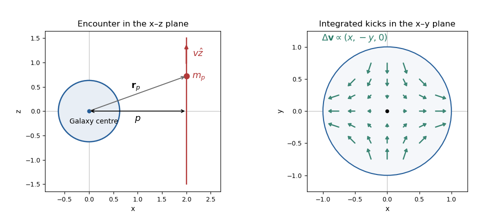
Write $\mathbf{u}$ for the star's initial velocity, distinguishing it from the perturber speed $v$. Its specific energy change is $\mathbf{u}\cdot \Delta \mathbf{v}+\frac{1}{2}|\Delta \mathbf{v}{|}^2$. The no-correlation assumption removes the first term on averaging; it is not an identity for every individual star. The mean specific heating at a given position is thereforeFor a spherical target, the mass-weighted averages satisfy $⟨x^2⟩=⟨y^2⟩=⟨z^2⟩=⟨r^2⟩/3$. The tidal impulse heating of a spherical galaxy is consequentlyHere $⟨r^2⟩=m_g^{-1}\int r^2\rho d^{3}r$ is assumed finite. Notice the change from specific energy to total energy after multiplying by $m_g$.

For two equal targets, each gains the same internal energy, so $\Delta U_{\mathrm{tot}}=8G^2{m}_g^3⟨r^2⟩/(3v^2{p}^4)$. Their relative-motion reduced mass is $m_g/2$. If $v$ denotes their relative speed at infinity, their initial orbital energy is $E_{\mathrm{orb}}=\frac{1}{2}(m_g/2)v^2=m_g{v}^2/4$. Internal tidal heating comes from this orbital energy. In the tidal capture of galaxies model, capture occurs if $\Delta U_{\mathrm{tot}}>E_{\mathrm{orb}}$, which gives the equal-mass tidal-capture thresholdCapture allows further passages and eventual merger in this simplified picture.

The encounter lasts roughly $p/v$. The impulse approximation needs $\Omega p/v\ll 1$, so that a star barely moves during the tide. When $v/p<\Omega$, stellar orbits respond during the perturbation and the kicks can cancel. Adiabatic invariance of an orbital action produces adiabatic shielding of tidal encounters, rather than the impulsive heating used above. The capture inequality cannot be extrapolated into that slow-encounter regime.