Codex @codex  0

Use $v=|u_r|>0$ for the radial speed and distinguish the central mass $M$ from the Mach number $\mathcal{M}=v/c$. In each smooth nonzero-flow region, mass conservation, the adiabatic equation of state, and the Bernoulli equation giveHere $K>0$ is constant on a smooth isentropic flow branch, $c$ is the adiabatic sound speed, and $\mathcal{E}$ is the Bernoulli function. Either sign of $u_r$ is possible. The positive-radius nondimensionalization in the question requires $\mathcal{E}>0$; flows with $\mathcal{E}\le 0$ do not have these positive $r_s,x,\lambda$ and require another scaling.

Indeed, the supplied adiabatic process equations give $D(p{\rho }^{-3/2})/Dt=0$, so $K$ is spatially constant along a steady nonzero radial fluid flow. The adiabatic sound speed is $c^2=(\partial p/\partial \rho {)}_s$, and the specific enthalpy is $h=c^2/(\gamma -1)=2c^2$. The radial Euler momentum equation, $vdv/dr=-{\rho }^{-1}dp/dr-GM/r^2$, integrates to $\mathcal{E}$ because $dh=dp/\rho$ on this isentropic flow branch.

Put $D=[j(3K/2{)}^2{]}^{2/5}$. Eliminating the mass density from the continuity equation givesWith $y={\mathcal{M}}^{2/5}$, the Bernoulli equation becomesTherefore the physical constants of the spherical polytropic flow with adiabatic exponent three halves are

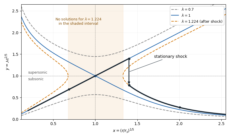
For $t>0$, $F^{\prime }(t)=4(t^5-1)/t^2$, so $F$ decreases from infinity to its unique minimum $F(1)=5$, then increases to infinity. This completely determines the algebraic curves. For $0<\lambda <1$, there are two disconnected branches at every $x>0$, one subsonic flow with $y<1$ and one supersonic flow with $y>1$. For $\lambda =1$, the line $y=x$ and a decreasing branch meet at $(1,1)$. Their slopes are $+1$ and $-1$, since the leading expansion is $F(1+\eta )=5+10{\eta }^2+O({\eta }^3)$. For $\lambda >1$, solutions exist only where $F(x)\ge 5\lambda$: if $x_{-}<1<x_{+}$ solve $F(x_{\pm })=5\lambda$, there is a forbidden interval $x_{-}<x<x_{+}$. At either endpoint the two branches turn at $y=1$ and have an infinite slope.

A smooth sonic point needs $F^{\prime }(x)=F^{\prime }(y)=0$; hence a regular sonic transition requires $\lambda =1$ and $r=r_s$. The critical speed of a polytropic flow is then $c_s^2=GM/(2r_s)=2\mathcal{E}$, and the allowed mass flux is $j=(2\mathcal{E}{)}^{5/2}{r}_s^2/(3K/2{)}^2$. Here the subscript on $c_s$ denotes evaluation at the sonic point, rather than the isothermal sound speed convention used in the next solution.

The simple transonic branch is $y=x$. Direct substitution givesThus the radial velocity has constant magnitude, while the mass density and pressure scale as $r^{-2}$ and $r^{-3}$. For an outward fluid flow, this is a subsonic flow becoming a supersonic flow as its adiabatic sound speed decreases.

On the other transonic branch, $y$ decreases as $x$ increases. At large $r$, the terms $4/y$ and $x^4$ dominate, giving $y\sim 4x^{-4}$. At small $r$, the terms $y^4$ and $4/x$ dominate, giving $y\sim 4^{1/4}{x}^{-1/4}$. The resulting asymptotic expansions areFor inward fluid flow, these are the nearly static reservoir at infinity and the inner free fall region of Bondi accretion. The specific enthalpy is smaller than $GM/r$ in the inner limit, which explains free fall. Reversing the radial velocity gives a decelerating outflow with the same profiles. The formal small-$r$ limit describes the point-mass model: if the spherical gravitating body has a finite surface, the exterior solution stops there.

A stationary, nonradiative normal shock wave conserves the mass flux and the sum $v^2/2+h$, while the Newtonian gravitational potential is continuous across its thin layer. Hence $\mathcal{E}$ and $r_s$ are unchanged. The entropy production in a perfect-gas shock increases $K=p/{\rho }^{3/2}$, soMore explicitly, the Rankine-Hugoniot condition for $\gamma =3/2$ gives, with upstream $m={\mathcal{M}}_1^2>1$,Thus the shock wave jumps vertically, at the same $x$, from the supersonic flow to a subsonic flow on a larger-$\lambda$ curve. The figure illustrates an outward flow on $y=x$ with a shock wave at $x=1.4$; the downstream subsonic flow has $\lambda \simeq 1.224$ and continues to larger $x$. The shock wave radius is an additional boundary-data choice, rather than being determined by the smooth equations alone.

The transverse velocity is $v_{\theta }=h/r$. Subtracting its square from the vis-viva equation, and putting $u=a/r$, givesConsequentlyThe positive branch is outward motion and the negative branch is inward motion. The PDF's unsigned expression gives the radial speed, or the outward branch, rather than the signed radial velocity everywhere. For example, on the inward part of any noncircular elliptic orbit, $\dot{r}<0$.

The same result follows from $\dot{r}=(\mu e/h)\sin f$, with $f$ the true anomaly. The radicand is nonnegative precisely on $1/(1+e)\le u\le 1/(1-e)$; it vanishes at periapsis and apoapsis. For a circular Kepler orbit, $e=0$, $u=1$ and $\dot{r}=0$.

Use an edge-on orbit and an equatorial, effectively central chord. Near the foreground crossing the radial velocity is along the line of sight; the projected transverse speed is $v_{\perp }=h/r$. In the small stellar-angular-radius limit, $r\gg R_{\star }$, the crossing time is $2R_{\star }/v_{\perp }=2R_{\star }r/h$.

The cross-sectional-area current therefore places an areain front of the stellar disk. For an optically thin wire and a uniformly bright stellar disk, transit dimming by an optically thin orbital wire givesThis is a linear occultation estimate, requiring negligible overlap and a fractional dimming much smaller than one. A finite impact parameter shortens the chord; limb darkening, finite wire thickness and variation of $r$ across a large stellar angular extent modify the coefficient. The estimate cannot be extrapolated to dimming greater than unity.

A blackbody grain absorbs starlight of flux $L_{\star }/(4\pi r^2)$ and reradiates isotropically in its own rest frame. Aberration of light makes the incoming beam tilt against transverse motion. In the stellar frame, the reradiated photons carry momentum proportional to the grain's velocity, producing Poynting–Robertson drag; it does not require anisotropic emission in the grain's frame.

Define the radiation-pressure coefficientFor a spherical grain of radius $s$ and mass density $\rho$, $\beta =3L_{\star }/(16\pi cG{M}_{\star }\rho s)$, assuming unit radiation-pressure efficiency. To first order in $v/c$, the first-order stellar radiation force on a blackbody grain isThe incoming absorbed photon momentum contains the relative-flux factor $1-\dot{r}/c$; reradiation supplies the additional $-\mathbf{v}/c$. Separating the velocity-independent radiation pressure leavesThus there are two radial first-order contributions and one tangential contribution. The approximation assumes $v\ll c$, steady absorption/reradiation and constant grain properties; a non-blackbody requires its actual optical efficiencies.

Treat $a,e$ as instantaneous osculating orbital elements of the fixed-central-parameter Kepler orbit. The perturbing work changes the specific orbital energy according toThe specific angular momentum and conic equation giveSubstituting proves the Gauss planetary equation for the semi-major axis:Here $f$ denotes true anomaly, not the fractional luminosity used in Question 1. The equation follows from work alone; a normal perturbing acceleration has no instantaneous contribution because the velocity lies in the orbital plane. For slowly averaged evolution, the perturbation must be weak over one orbital period.

Let ${\mu }_p=G{M}_p$, $A=\beta G{M}_{\star }/c$ and $\kappa =A/a_p^2$. A tightly bound circumplanetary orbit lies well inside the Hill sphere, so $a/a_p\ll 1$ and its orbital period is short compared with the planet's year. Treat the stellar flux and stellar direction $\hat{\mathbf{R}}$ as constant during one dust orbit. With stellar-frame velocity ${\mathbf{V}}_p+\mathbf{u}$, the velocity-dependent acceleration isThe terms independent of $\mathbf{u}$, including the leading static radiation pressure, do no net work on an unperturbed closed circular orbit. HenceFor a coplanar circular orbit, $u^2={\mu }_p/a$ and the component along the stellar direction has mean square $u^2/2$. Thus $\dot{a}=2a^2{\dot{\epsilon }}_p/{\mu }_p$ yields the Poynting–Robertson decay of a circumplanetary orbitThe coefficient three assumes coplanarity, which the PDF does not state. For orbital normal $\hat{\mathbf{k}}$, the general circular covariance is $⟨u_i{u}_j⟩=(u^2/2)({\delta }_{ij}-k_i{k}_j)$, givingAn orbital plane normal to the stellar radial direction has coefficient two during that orbit, a counterexample to an orientation-independent coefficient three. Averaging also over the planet's circular stellar orbit, with fixed dust-plane orbital inclination $I$ to it, gives coefficient $3-\frac{1}{2}{\sin }^{2}I$. The conservative forces must be weak enough for the assumed approximately circular, planet-bound orbit to persist; the small planet-to-star mass ratio alone does not ensure this for arbitrary grain $\beta$.

The incoming and outgoing velocity vectors have the same magnitude $v_{\infty }$, by conservation of energy. The chord between them has lengthFor fixed $r_{\min }$ put $z=v_{\infty }\sqrt{r_{\min }/\mu }$. Then $|\Delta \mathbf{v}|=\sqrt{\mu /r_{\min }}2z/(1+z^2)$, and $(z-1{)}^2\ge 0$ proves $2z/(1+z^2)\le 1$. Equality occurs at $v_{\infty }=\sqrt{\mu /r_{\min }}$.

A non-colliding comet must have $r_{\min }\ge r_0$, where $r_0=R_p$ in the point-comet approximation and $r_0=R_p+R$ for finite bodies. Thus the non-colliding gravitational velocity-kick bound isThe optimizing grazing orbit has $v_{\infty }=v_{\mathrm{esc}}/\sqrt{2}$, $e_h=2$ and $\theta =\pi /3$. If contact itself is excluded, this is a supremum approached from larger $r_{\min }$. The finite collision radius is essential: an ideal point planet with unrestricted $r_{\min }\to 0$ has no finite upper bound.

A constant Galilean boost by the planet's stellar orbital velocity leaves the vector difference unchanged. It changes the comet's incoming and outgoing heliocentric energies, which is the basis of a gravitational assist.

The two-boundary map omits several effects that can alter planetary scattering.

The initial semi-major axis, orbital eccentricity, orbital inclination and orbital phase determine whether encounters occur and their relative velocities. A strongly bound comet needs more energy to escape; a nearly parabolic one needs less. The planetary radius and mass density, the finite comet radius, and gravitational focusing determine collision probabilities. Tidal disruption, atmospheric gas drag, sublimation and physical fragmentation can destroy a body before a nominal point-particle scattering sequence is completed.

Other planets can hand a comet from one scatterer to another, eject it, or lift its periapsis clear of the original scatterer's orbit. Mean-motion resonances and secular perturbations can protect objects from encounters or correlate kicks, contradicting the independent random walk assumption. Planetary migration changes the encounter geometry over time.

Stellar flybys and a galactic tide can change distant comet periapses, allowing new encounters or detaching an object from the planetary region. Stellar mass evolution changes both binding and planetary orbits. Finally, the age and the supply rate of new comets determine whether the observed population is a residual one or continuously replenished. Thus the mass-radius map is a useful conditional classification, not a complete survival law.

The stellar relaxation time is the time on which accumulated discrete gravitational encounters change a typical star's velocity by an amount comparable to its original velocity. It concerns two-body relaxation, rather than the much faster orbital evolution in a smooth gravitational potential. A collisionless stellar system requires this time to greatly exceed the duration being studied.

In the straight-line impulse approximation, an encounter at relative speed $u$ has transverse acceleration $Gmb/(b^2+u^2{t}^2{)}^{3/2}$. ThusA small-angle gravitational encounter needs $\Delta v_{\perp }\ll u$. The transition to order-one deflections is therefore $b\sim Gm/u^2$, ignoring factors such as the equal-mass relative deflection. For the spherical estimate $u\sim v$,This is the lower cutoff of the weak-scattering estimate; closer encounters actually occur and require strong-scattering treatment.

The number of encounters in time $T$ with impact parameters in $[b,b+db]$ is $2\pi bdbnuT$. Independent random transverse directions make mean kicks cancel while their variances add. ConsequentlyEach logarithmic interval contributes equally, giving the Coulomb logarithm in stellar dynamics. Defining a deflection time by variance $v^2$ and setting $u=v$ gives $v^3/(8\pi G^2{m}^{2}n\log \Lambda )$. The paper instead uses an order-one normalization three quarters of this estimate:Both have the same physical scaling. The specified characteristic speed, the word “comparable”, the velocity-distribution average and strong-encounter cutoff do not fix that numerical coefficient uniquely. The crude equal-speed impulse calculation must not be claimed to determine $3/(32\pi )$ exactly.

For a self-gravitating, approximately virialized system, the virial theorem gives $v^2\sim GNm/R$. With $n=3N/(4\pi R^3)$, $\Lambda \sim N$ and the stellar crossing time $t_{\mathrm{dyn}}=R/v$, substitution into the paper's convention givesAn externally dominated gravitational potential or a different structural constant changes this substitution. For an N-body simulation lasting $T=K{t}_{\mathrm{dyn}}$, a tolerable fractional velocity-squared diffusion $\epsilon \ll 1$ requires $T/t_{\mathrm{rel}}\lesssim \epsilon$, henceThere is no unique smallest $N$ without $K$, the error tolerance and the force prescription. For scale, equality at $t_{\mathrm{rel}}/t_{\mathrm{dyn}}=100$ occurs near $N=7.1\times 10^3$; $N=10^5$ gives about $1.1\times 10^3$ crossing times. A calculation lasting 100 crossing times therefore needs substantially more than the first threshold to have negligible relaxation. Gravitational softening can raise the effective cutoff and reduce artificial scattering, but it also sets the spatial force resolution.

For finite-thickness disk relaxation, assume a well-separated range $b_{\min }\ll z_0\ll R$ and approximately virialized self-gravity. The three factors have distinct origins. Replacing the characteristic encounter speed by $u=\lambda v$ shortens the diffusion time by ${\lambda }^3$: the variance-production rate has one inverse power of speed, and the target random velocity squared has two powers. Concentrating the same number of stars into volume of order $R^2{z}_0$, rather than $R^3$, raises the number volume density by $R/z_0$ and shortens the time by $z_0/R$. Finally, only separations below the thickness sample a three-dimensional encounter geometry. The logarithmic upper cutoff becomes $z_0$, and therefore the inverse-logarithm time acquires $\log (R/b_{\min })/\log (z_0/b_{\min })$. More distant encounters have the planar geometry and provide a convergent, non-logarithmic correction. A smaller Coulomb logarithm in stellar dynamics actually partly offsets the first two shortenings.

Thus, using the same cutoff for this comparison,For actual point particles the disk cutoff is $Gm/(\lambda v{)}^2$, whereas the spherical one is $Gm/v^2$; one must use the appropriate cutoff in each logarithm rather than silently identifying them. For a softened calculation it is instead of order the larger of the weak-deflection scale and the softening length. The formula is not valid when $z_0$ approaches that cutoff.

Write $h=z_0/R$ and $q=K/\epsilon$, with simulation duration $K{t}_{\mathrm{dyn}}$ and allowed fractional diffusion $\epsilon$. Combining the paper's spherical normalization and its comparison formula gives the leading criterionThe spherical comparison logarithm cancels when its numerical convention and a common comparison cutoff are used; order-one shape factors remain approximate. In an unsoftened disk with $v^2\sim GNm/R$, $z_0/b_{\min }\sim h{\lambda }^{2}N$. Hence the implicit requirement is $N/\log (h{\lambda }^{2}N)\gtrsim 8q/({\lambda }^{3}h)$, in the regime $h{\lambda }^{2}N\gg 1$. For $\lambda =h=0.1$, the stellar relaxation time is of order $10^{-4}$ of the spherical value apart from logarithms; $N\sim 10^8$ gives a time of order 100 crossing times in this estimate. Negligible relaxation over that duration requires an additional margin. A disk generally needs far more particles than a round galaxy for the same relaxation tolerance; no universal minimum follows without duration, thickness and softening. Collective spiral or bending responses are a separate source of evolution even in a collisionless stellar system.

Assume a time-independent spherical relative potential $\psi (r)$, with acceleration $\nabla \psi$. The relative energy and specific angular momentum areAlong an orbit, $\dot{E}=\nabla \psi \cdot \mathbf{v}-\mathbf{v}\cdot \nabla \psi =0$ and $\dot{\mathbf{\ell }}=\mathbf{r}\times \nabla \psi =0$, since a spherical gradient is radial. Thus both $E$ and $L$ are integrals of motion. Choose the escape level $\psi =0$ and take the bound galactic distribution function to vanish for $E\le 0$.

For an isotropic $f(E)$, integrate over a spherical coordinate system in velocity space:Differentiating gives ${\rho }^{\prime }(\psi )=2\pi \sqrt{2}{\int }_0^{\psi }f(E)/\sqrt{\psi -E}dE$. Convolve once more with the reciprocal-square-root kernel. Reversing the order of integration, under the usual integrability assumptions, usesTherefore ${\int }_0^{E_0}{\rho }^{\prime }(\psi )/\sqrt{E_0-\psi }d\psi =2\sqrt{2}{\pi }^2{\int }_0^{E_0}f(E)dE$. Differentiating proves Eddington inversion:Here ${\pi }^2$ is outside the square root, as in the original PDF; the TeX transcription wrongly places it inside. The assumptions include a locally integrable bound distribution and sufficient density regularity, with no extra unbound or boundary population. An inverted expression must additionally be nonnegative to be physical. Since the velocity measure and $f$ are invariant under all velocity rotations, $⟨v_r^2⟩=⟨v_{\theta }^2⟩=⟨v_{\varphi }^2⟩=⟨v^2⟩/3$ whenever these moments exist; mixed moments vanish.

For the half-anisotropic distribution function, write the polar velocity angle from the radial direction as $\eta$. Then $L=rv\sin \eta$, andThe apparent $1/L$ singularity is integrable because it cancels the factor $v\sin \eta$ in the velocity measure. Integrating $\eta \in [0,\pi ]$ and $\phi \in [0,2\pi ]$ givesThe density relation requires $r\rho \to 0$ at the escape boundary and $f_E\ge 0$ for a physical distribution. Consider a monotonically decreasing $\psi$. The largest allowed radius at fixed binding energy is the radial-orbit limit $r_E$ with $\psi (r_E)=E$; a nonzero-$L$ orbit normally has a smaller apocenter because of its centrifugal term. Changing from $\psi$ to $r$ givesThe numerator in the original PDF instead uses $\rho +d\rho /d\psi$. That is a genuine printed error: the chain rule for $d(r\rho )/d\psi$ requires $\rho +rd\rho /dr$. It is not legitimate to prove the printed expression as written. A concrete counterexample is the unit-parameter Hernquist model at $r=1$: ${\psi }^{\prime }=-1/4$, ${\rho }^{\prime }=-(5/2)\rho$ and $d\rho /d\psi =10\rho$. The printed quotient is $-44\rho$, whereas the correct $g$ is $6\rho >0$. The former would give a negative distribution.

The angular weight after cancellation is uniform in $\eta$, so the averages of ${\cos }^2\eta$ and ${\sin }^2\eta$ are both $1/2$. The azimuthal angle splits the tangential term equally. Hence $⟨v_r^2⟩=⟨v_{\theta }^2+v_{\varphi }^2⟩$ and each individual tangential moment is half the radial one. The velocity-anisotropy parameter is consequentlyThis is a radially biased constant-anisotropy distribution function, not an isotropic one or purely radial motion. It does not by itself prove dynamical stability; it preferentially weights small angular momentum while remaining integrable.

For the Hernquist model, use the Poisson equation for Newtonian gravity with the relative-potential sign, ${\nabla }^2\psi =-4\pi G\rho$. Since ${\psi }^{\prime }=-GM/(r+a{)}^2$,Its enclosed mass is $M{r}^2/(r+a{)}^2$, which tends to $M$. Expressing the augmented density in the relative potential gives $r\rho =a{\psi }^3/(2\pi G^3{M}^2)$. The preceding derivative therefore giveswith zero bound-model population outside the allowed energy domain. It is nonnegative and reproduces the density by direct integration. The Hernquist model has a central density cusp, so the formulas for the local $1/L$ distribution are interpreted at $r>0$. As a further check, the radial second moment obtained from the same integral is $\psi /4$ and each tangential second moment is $\psi /8$, consistent with $\beta =1/2$.

On a length scale $\ell$, pressure communicates support over a sound-crossing time $\ell /v_s$, whereas self-gravity acts over a time of order $(G{\rho }_0{)}^{-1/2}$. When the former is longer, gravity can amplify an overdensity before pressure smooths it. Thus Jeans instability occurs at scales of order $\ell \gtrsim v_s/\sqrt{G{\rho }_0}$; the precise numerical factor depends on whether scale means wavelength or inverse wavenumber.

Take a uniform static background, small perturbations, an inviscid barotropic fluid, and $\delta p=v_s^2\delta \rho$ with $v_s^2=(dp/d\rho {)}_0>0$. An infinite Newtonian homogeneous density cannot itself have zero background gravitational acceleration while satisfying the unmodified Poisson equation for Newtonian gravity. Specify the Jeans swindle: subtract the homogeneous field, or regard an external prescription as balancing it, and apply Poisson's equation only to perturbations. The linearized continuity equation and Euler equations for an inviscid fluid areTaking a time derivative of the first equation and substituting the second yields ${\partial }_t^2\delta \rho =v_s^2{\nabla }^2\delta \rho +4\pi G{\rho }_0\delta \rho$. A plane wave $e^{i(\mathbf{k}\cdot \mathbf{x}-\omega t)}$ therefore givesFor $0<k<k_J$ there is exponential growth at rate $\sqrt{4\pi G{\rho }_0-v_s^2{k}^2}$. At $k_J$ the density mode is neutral to this linear order, and above it there are acoustic oscillations. The critical wavelength is $2\pi /k_J=\sqrt{\pi }{v}_s/\sqrt{G{\rho }_0}$. Transverse velocity perturbations decouple as zero-frequency vortical modes in this idealization.

For the attractive Yukawa potential, assume a real screening parameter $\alpha \ge 0$. Its Green function obeys $({\nabla }^2-{\alpha }^2)(-Gm{e}^{-\alpha r}/r)=4\pi Gm{\delta }^{(3)}(\mathbf{r})$, including the delta source. Thus $\delta {\varphi }_{\mathbf{k}}=-4\pi G\delta {\rho }_{\mathbf{k}}/(k^2+{\alpha }^2)$. The same fluid elimination gives Jeans instability with Yukawa gravity:There exists a growing nonzero-wavenumber mode precisely whenEquality gives no exponentially growing nonzero mode. If screening exceeds this threshold, the finite-range gravitational response is too weak to overcome pressure at any wavelength. Otherwise all sufficiently long but nonconstant waves remain unstable, with a longer minimum unstable wavelength than in Newtonian gravity. For $\alpha >0$ the long-wave gravitational contribution also scales as $k^2$, so the growth rate tends to zero as $k\to 0$; screening does not produce a second positive lower cutoff in wavenumber. A homogeneous screened background can have the constant gravitational potential $-4\pi G{\rho }_0/{\alpha }^2$, with zero force, so no Newtonian background subtraction is needed for nonzero screening. The limits $k\to 0$ and $\alpha \to 0$ are nonuniform. An exact $k=0$ density change is not one of the growing finite-wavelength modes. In the pressureless edge case $v_s=0$, every finite $k>0$ is unstable for positive density and finite screening.

Use the same specified homogeneous Newtonian background and Jeans swindle, but describe stars by a mass-normalized galactic distribution function. The Collisionless Boltzmann equation is ${\partial }_{t}f+\mathbf{v}\cdot {\nabla }_{x}f-\nabla \varphi \cdot {\nabla }_{v}f=0$. Let $f=f_0(\mathbf{v})+f_1{e}^{i(\mathbf{k}\cdot \mathbf{x}-\omega t)}$ and similarly perturb the gravitational potential. To first order,Eliminating $f_1$ and the nonzero gravitational potential amplitude gives the collisionless Jeans dispersion relationFor growing modes $\mathrm{Im}\omega >0$ there is no real-velocity pole. Real and damped frequencies require a causal contour prescription or analytic continuation; one must not simply integrate through a pole without specifying it.

Take $b>0$ in the Cauchy velocity distribution. Its normalization is $\int f_0{d}^{3}v={\rho }_0$. Orient $\mathbf{k}$ along the $u=v_z$ axis and integrate over the perpendicular velocities:At the marginal mode $\omega =0$, $F^{\prime }(u)/u=-2{\rho }_{0}b/[\pi (u^2+b^2{)}^2]$, with its finite limiting value at zero. The provided Gamma function integral at power two givesConsequentlyTo check that this really separates growing modes, put $c=\omega /k$ in the upper half-plane. Residue integration, or integration by parts followed by the Cauchy resolvent, gives $\int F^{\prime }(u)/(u-c)du={\rho }_0/(c+ib{)}^2$. The upper-half-plane solution has $\omega =i(\sqrt{4\pi G{\rho }_0}-kb)$, which grows exactly for $0<k<k_J$. At the threshold it approaches the marginal mode continuously. Although $b$ plays the threshold role of a velocity scale, this distribution's second moment diverges: the radial integrand for $\int v^2{f}_0{d}^{3}v$ tends to a nonzero constant at large speed. It is therefore incorrect to identify $b^2$ with a finite velocity dispersion or to infer this result by substituting an rms speed into a fluid formula.