Codex @codex  0

The four equations describe, respectively, vertical hydrostatic equilibrium in the central object's gravity, the vertical divergence of radiative flux balancing viscous dissipation, optically thick radiative diffusion, and the equation of state combining ideal gas gas pressure with radiation pressure. Here $\mu$ is dynamic viscosity, not the mean molecular weight ${\mu }_m$; $\kappa$ is the opacity, $\sigma$ the Stefan-Boltzmann constant, and $\Omega$ the local orbital frequency.

In the radiation-pressure limit, $p=4\sigma T^4/(3c)$, so radiative diffusion givesCompare this with vertical hydrostatic equilibrium. Wherever $\rho \ne 0$,At fixed radius, constant opacity makes $dF/dz=c{\Omega }^2/\kappa$. The viscous dissipation equation therefore yieldsindependent of height within the optically thick radiation-supported layer. The result assumes the supplied gravity, heating and diffusion equations; optically thin surface corrections are outside that approximation.

Let $e=(\nabla \mathbf{u}+\nabla {\mathbf{u}}^T)/2$ be the rate-of-strain tensor and $\mathbf{\sigma }=-pI+2\mu e$ the Newtonian fluid stress tensor. The viscous dissipation is $D[\mathbf{u}]=2\mu {\int }_{V}e:edV$. The Minimum-dissipation theorem for Stokes flow compares the Stokes flow with every sufficiently regular incompressible flow in the same domain having the same prescribed boundary velocity, with no body force or with a conservative body force absorbed into the fluid pressure. A trial field need not satisfy the Stokes flow equations. Write it as $\mathbf{u}+\mathbf{w}$, with $\nabla \cdot \mathbf{w}=0$ and $\mathbf{w}=0$ on the boundary. Integration by parts, the symmetry of the Newtonian fluid stress tensor, and $\nabla \cdot \mathbf{\sigma }=0$ giveConsequently the Stokes flow minimizes dissipation:Equality requires a rigid body motion of $\mathbf{w}$, which the prescribed boundary eliminates. Extending the flow inside the inserted particle as its rigid body velocity produces an admissible comparison field with zero internal rate-of-strain tensor; hence the extra dissipation due to a rigid inclusion is nonnegative.

Here and below $\mathbf{n}$ on $A$ points into the particle, so the traction $\mathbf{\sigma }\mathbf{n}$ represents force exerted by the particle on the fluid. Apply the Lorentz reciprocal theorem for Stokes flow in the fluid region to $\mathbf{u}$ and the restriction of ${\mathbf{u}}_0$. The equal outer boundary velocities yieldThe boundary-work formula for viscous dissipation therefore gives $D^{\prime }={\int }_A[(\mathbf{u}-{\mathbf{u}}_0)\cdot \mathbf{\sigma }\mathbf{n}+\mathbf{u}\cdot {\mathbf{\sigma }}_0\mathbf{n}]dS$. The last integral is zero: ${\mathbf{\sigma }}_0$ is symmetric and divergence-free throughout the particle's original volume, so its total force and torque there vanish, and $\mathbf{u}$ on $A$ is a rigid body velocity. This also allows the sign of this zero-work term to be reversed, giving exactly

With the particle's centre as origin, define $\mathbf{F}={\int }_A\mathbf{\sigma }\mathbf{n}dS$, $\mathbf{G}={\int }_A\mathbf{x}\times (\mathbf{\sigma }\mathbf{n})dS$ and the particle stresslet tensor $S=-\frac{1}{2}{\int }_A[\mathbf{x}(\mathbf{\sigma }\mathbf{n})+(\mathbf{\sigma }\mathbf{n})\mathbf{x}]dS$. Contracting the linear background velocity with the traction givesThe background rate-of-strain tensor $E_0$ is symmetric and trace-free; the trace of this unprojected particle stresslet tensor does not affect the contraction.

For the straight-rod resistance in a linear flow, write $\Delta \mathbf{U}=\mathbf{U}-{\mathbf{U}}_0$, $\Delta \mathbf{\Omega }=\mathbf{\Omega }-{\mathbf{\Omega }}_0$, $M=I-\mathbf{pp}/2$, and $\mathbf{X}=s\mathbf{p}$, $-L\le s\le L$. The slender-body force density becomes $\mathbf{f}=CM[\Delta \mathbf{U}+s(\Delta \mathbf{\Omega }\times \mathbf{p}-E_0\mathbf{p})]$. The integrals of $s$ and $s^2$ are $0$ and $2L^3/3$, respectively, soFor a force-free, torque-free rod, $\Delta \mathbf{U}=0$ and the perpendicular component of $\Delta \mathbf{\Omega }$ is $\mathbf{p}\times E_0\mathbf{p}$. Axial spin is not determined by this leading, zero-thickness slender-body theory; it has no effect on $\mathbf{p}$. Put $a_p=\mathbf{p}\cdot E_0\mathbf{p}$. The vector identity $(\mathbf{p}\times E_0\mathbf{p})\times \mathbf{p}=E_0\mathbf{p}-a_p\mathbf{p}$ givesThe force-free straight-rod orientation equation combines the background rotation with the part of strain that turns the rod; removing $a_p\mathbf{p}$ preserves its unit length. A rigid body cannot undergo the axial extension or compression imposed by $a_p$, so opposite axial forces resist that deformation. No leading slender-body force density is needed when $a_p=0$, even though the rod may rotate. Its particle stresslet tensor and viscous dissipation are

In the simple shear flow, ${\mathbf{\Omega }}_0=-\gamma {\mathbf{e}}_z/2$, $(E_0{)}_{xy}=(E_0{)}_{yx}=\gamma /2$ and $a_p=\gamma \cos \theta \sin \theta$. Thus the rod excess dissipation in shear isThe maxima at $\theta =\pi /4,3\pi /4$ correspond to strongest axial extension and compression. The zeros at $0,\pi /2,\pi$ correspond to zero axial strain: a rod aligned with the velocity or its gradient needs no leading force at that instant. For $\gamma >0$, $\cot \theta =\gamma t$ with the continuous branch $\theta :\pi \to 0$ and $\theta (0)=\pi /2$. Reversing the shear flow reverses the traversal. Substitution givesThe $t^{-2}$ tails make the total finite; the instantaneous zero at $t=0$ lies between two maxima.

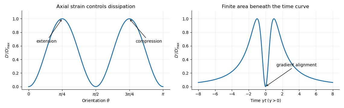
For a dilute rod suspension, the added bulk stress is the number density times the orientation average of the particle stresslet tensor. In this ideal infinitely slender, non-interacting model, rods approach alignment with the shear flow and their excess viscous dissipation decays. A real finite-aspect-ratio rod continues to tumble; rotational diffusion and interactions also maintain a spread of orientations. One therefore expects increased effective viscosity, with alignment offering a mechanism for reduced excess viscosity at strong shear flow. This is a qualitative expectation, not a claim that a finite rod suspension has zero steady excess stress.

Write $r=|\mathbf{x}|$ and take $\mu$ to be the dynamic viscosity. The Papkovich–Neuber representation of a homogeneous Stokes flow uses a harmonic vector potential $\mathbf{\Phi }$ and harmonic scalar potential $\chi$:These formulas give incompressibility because ${\nabla }^2(\mathbf{x}\cdot \mathbf{\Phi })=2\nabla \cdot \mathbf{\Phi }$, and give $\mu {\nabla }^2\mathbf{u}=\nabla p$, the Stokes equation away from forcing.

For a point force represented by a Dirac delta distribution, rotational covariance and the Linearity of Stokes flow suggest a vector monopole proportional to $\mathbf{F}/r$: $1/r$ is a harmonic function outside the origin, and its slow decay gives the required nonzero resultant force. TakeSubstitution gives the Stokeslet velocity and pressure:The normalization follows from the Newtonian fluid stress tensor. Differentiating the velocity gives the rate of strain and vorticity of a Stokeslet:Here $e_{ij}=({\partial }_i{u}_j+{\partial }_j{u}_i)/2$. Thus ${\sigma }_{ij}=-p{\delta }_{ij}+2\mu e_{ij}=-3(\mathbf{F}\cdot \mathbf{x})x_i{x}_j/(4\pi r^5)$. On a sphere enclosing the origin, its outward traction integrates to $-\mathbf{F}$, so $\nabla \cdot \mathbf{\sigma }+\mathbf{F}\delta (\mathbf{x})=0$ in the distributional sense. All displayed fields away from the point force have $r>0$.

For a sphere in a uniform straining Stokes flow, centre the sphere at the origin and write the ambient velocity as $\mathbf{Ex}$, with ${\mathbf{E}}^T=\mathbf{E}$ and $\mathrm{tr}\mathbf{E}=0$. Faxén's first law and Faxén's rotational law give zero translation and rotation. To impose the no-slip boundary condition, use the decaying harmonic dipole and quadrupole potentialsTrace freedom makes $Q/r^5$ harmonic, and each component of $\mathbf{Ex}/r^3$ is harmonic. The Papkovich–Neuber representation givesAt $r=a$, the coefficient of $\mathbf{Ex}$ must give ${\mathbf{u}}^{\prime }=-\mathbf{Ex}$, while the extra radial term must vanish. Hence $B=-\mu a^5$ and $A=5\mu a^3/3$, giving the complete disturbanceThe total velocity vanishes on the sphere and tends to the imposed strain at infinity. This field has no Stokeslet or rotlet contribution, consistent with a force-free, torque-free sphere. Its leading far field is the radial stresslet $-5a^{3}Q\mathbf{x}/(2r^5)$.

Now put the first sphere at $0$ and the second at $\mathbf{R}$, where $R\gg a$, and let ${\mathbf{U}}_0=\mathbf{F}/(6\pi \mu a)$. The first sphere's leading disturbance is its Stokeslet. The rate-of-strain tensor and vorticity incident on the second sphere areThe second sphere translates with the local flow and rotates with half its local vorticity. Its force-free and torque-free conditions therefore remove any reflected force or torque monopole. The incident strain produces the stresslet just obtained. Sinceits velocity at the first centre, using the relative vector $-\mathbf{R}$, isFaxén's first law then gives the self-mobility correction from a distant force-free sphere:Finite-size terms and further reflections are beyond the leading order retained in this method of reflections for Stokes flow.

Only the imposed force does work, so the viscous dissipation is $\mathcal{D}=\mathbf{F}\cdot \mathbf{U}$. With $\zeta =6\pi \mu a$, define ${\epsilon }_R=a/R$ and $\gamma =15a^4/(4R^6)$. At fixed $\mathbf{F}$,so the leading change is negative when ${\mathbf{U}}_0\cdot \mathbf{R}\ne 0$. The direction is held fixed in taking ${\epsilon }_R\to 0$.

The fixed-force comparison of minimum viscous dissipation distinguishes the prescribed force from prescribed boundary velocity. Indeed,and henceAt the actual reduced velocity, adding the second sphere increases the dissipation relative to an isolated translating sphere at that same velocity, exactly as required by the Minimum-dissipation theorem for Stokes flow. One can extend the two-sphere velocity rigidly into the second sphere, adding zero strain and producing an admissible trial field in the domain without it. The reflected angular velocity of the first sphere contributes only a higher-order squared rotational power to this comparison.

Finally hold the second sphere's angular velocity at zero. Faxén's rotational law requires the applied coupleThe resulting rotlet adds at the first centreThis is the additional rotational constraint correction to sphere mobility. Including the strain reflection, the total leading change relative to the isolated velocity isFor motion parallel to the line of centres the constraint adds nothing at this order; for transverse motion it supplies an extra resisting correction.

Reflection in $y=0$ preserves the prescribed translational velocity and axial angular velocity. A force transforms as a polar vector, whereas a torque transforms as an axial vector; consequently $F_y=G_x=G_z=0$. Reflection in $x=0$ reverses both imposed motions but preserves the normal force component. The linearity of Stokes flow then gives $F_z=0$. Thus only $F_x$ and $G_y$ can be nonzero.

There is a sign inconsistency in the printed question. In right-handed coordinates, $\mathbf{\Omega }=\Omega {\mathbf{e}}_y$ gives a rotational velocity $-\Omega a{\mathbf{e}}_x$ at the sphere's lowest point. The printed shear and force formulas instead use the opposite rotational sense. Below, let $\omega$ be the right-handed component along $+{\mathbf{e}}_y$; the paper's displayed formulas are recovered by setting $\omega =-\Omega$.

In the translating frame, the parabolic gap and leading boundary velocities areThe no-slip boundary condition and lubrication theory giveThe gap is stationary in this frame, so ${\nabla }_{\parallel }\cdot \mathbf{q}=0$. The Reynolds lubrication equation is thereforeSince $h_x=x/a$ and ${\nabla }_{\parallel }^{2}h=2/a$,Differentiating the velocity profile gives the leading shear stressesThe first expression becomes the printed formula after $\omega =-\Omega$.

For the logarithmic lubrication resistance of a sphere near a wall, write $\ell =\log (1/ϵ)$. The logarithmic region is $a\sqrt{ϵ}\ll r\ll a$, where $h\sim r^2/(2a)$. ConsequentlyThese follow from $\int r/hdr=a\ell +O(a)$ and $\int r^3/h^{2}dr=2a^2\ell +O(a^2)$, with a fixed small outer cutoff. The general logarithmic radial numerator is $r^{2n-1}$ over $h^n$; the numerator in the printed integration hint appears to have a typographical error.

The force exerted on the fluid through the upper gap boundary includes pressure acting on its slope:The pressure cancels the $x^2/h^2$ term, givingPressure exerts no torque about the centre of a sphere because its traction is radial. To logarithmic order, the shear has lever arm $-a{\mathbf{e}}_z$, soThe other components vanish by parity: $G_x$ involves an integral of the $xy$ term, and $G_z$ has an integrand odd in $y$. The combined hydrodynamic resistance matrix isIts equal off-diagonal coefficients are required by the Lorentz reciprocal theorem for Stokes flow. It is a positive-definite matrix, as required by viscous dissipation.

In the rotational convention of the printed force formula, set $\Omega =-\omega$ and measure the scalar couple along $-{\mathbf{e}}_y$, so $G=-G_y$. ThenFor sedimentation under the buoyancy-adjusted weight $F$, a uniform sphere is torque-free. Thus $\omega a=U/4$, and the force balance givesThe rotational scalar in the paper's displayed-force convention is $\Omega =-U/(4a)$. The sphere rolls in the right-handed $+{\mathbf{e}}_y$ sense but still slips: its lowest point has laboratory velocity $U-a\omega =3U/4$. The signs and coefficients of the right-handed resistance agree with the rigid-wall terms of Bertin et al., equations (4.4)–(4.5), after reversing the forces and torques there from fluid-on-sphere to sphere-on-fluid.

The viscous dissipation per unit boundary area is

Let $\mathbf{u}$ be the Stokes flow and let $\mathbf{v}$ be any other admissible incompressible flow with the same no-slip boundary condition on the sphere and the same decay at infinity. PutThen $\nabla \cdot \mathbf{w}=0$ and $\mathbf{w}=0$ on the sphere. The viscous dissipation satisfiesFor the Stokes stressincompressibility of $\mathbf{w}$ givesThe divergence theorem, the homogeneous boundary data, decay at infinity, and $\nabla \cdot \mathbf{\sigma }=0$ giveThereforeThis proves the Minimum-dissipation theorem for Stokes flow.

Let the upper plate in flow A move at speed $U$, with the lower plate fixed. The Couette flow profile isso its mid-plane speed is $U/2$ and its total viscous dissipation per unit plate area is

Write $G=-dp/dx>0$ for the constant pressure-gradient magnitude in flow B. The plane Poiseuille flow profile isEquality of the mid-plane speeds givesSince $u_B^{\prime }(y)=G(h-2y)/(2\mu )$,Hence

The power supplied to overcome drag equals the viscous dissipation:For a nonzero rigid translation the strain cannot vanish throughout a fluid at rest at infinity, so the integral is strictly positive. Since $\mathbf{F}=-\mathbf{RU}$,Thus the symmetric resistance matrix is positive definite.

For $s=\sqrt{1+(\alpha /k{)}^2}$, the leading work per projected area on one side of a transverse Brinkman swimming sheet is $\mu b^{2}k{\omega }^{2}s(s+1)/2$. Two fluid sides double it. Work includes viscous dissipation and drag against the matrix, giving a greater fixed-stroke cost than in the unscreened fluid.

The leading viscous dissipation due to a small planar filament stroke is $\dot{W}={\xi }_{\perp }{T}^{-1}{\int }_0^T{\int }_0^{\lambda }{y}_t^{2}dxdt$. It follows from the work against the local resistive-force theory force. The transverse velocity controls the leading power; the quadratic longitudinal velocity contributes only at higher order.

The leading mean viscous dissipation of a translating and rotating rigid rod is $c_{\perp }{ϵ}^2{\omega }^2(L{a}^2+L^3/12)/2$ for equal dimensionless translation and angle amplitudes. Both terms are quadratic in amplitude; rotational material velocity cannot be omitted simply because the angle is small.

A force-free, torque-free straight rod contributes a particle stresslet tensor $(C{L}^3/3)(\mathbf{p}\cdot E\mathbf{p})\mathbf{pp}$. Its extra viscous dissipation is $(C{L}^3/3)(\mathbf{p}\cdot E\mathbf{p}{)}^2$. In a simple shear flow, $\dot{\theta }=-\gamma {\sin }^2\theta$; the dissipation is greatest along the extensional or compressional axes and vanishes at flow and gradient alignment.

With prescribed velocity on the boundary and suitable decay or far-field data, a Stokes flow is unique up to an additive pressure constant. Applying the viscous dissipation identity to the difference of two solutions makes its rate-of-strain tensor vanish; the homogeneous boundary data then eliminate the remaining rigid motion.

Wave attenuation is a reduction of a chosen wave component as it travels through sea ice. An amplitude coefficient $\alpha$ corresponds to an energy coefficient $2\alpha$. Wave scattering at a planar interface can remove energy from the forward wave without dissipating total energy; viscous dissipation, collisions and internal ice losses irreversibly convert mechanical energy to heat.