Impedance bridging, also called voltage bridging, connects a source to a much higher load impedance so that little signal electric potential difference is lost across the source's output impedance. It is useful when the receiver should observe a signal while drawing little electric current from its source.
Represent a linear source at one frequency by open-circuit phasor and series electrical impedance . With receiving input impedance , the voltage divider givesThus makes close to one as a complex number, controlling both amplitude and phase loading. For positive electrical resistances, the relative voltage loss is . A source feeding retains of its open-circuit voltage; feeding retains .
For a tolerance on that resistive relative loss,The often convenient ten-to-one ratio is therefore a chosen accuracy compromise, not a universal definition. A one-percent limit requires at least a ninety-nine-to-one ratio in this ideal resistive model. Voltage divider loading error gives the related loading problem when the source is itself a divider.
Impedance bridging with capacitive input explains why a large DC electrical resistance is not enough at every frequency. With source resistance and receiving in parallel with capacitance ,At and , the DC ratio is about . With , its magnitude at is only about . The capacitive path loads the source despite the high DC input resistance.
Texas Instruments' three-amplifier presentation motivates high-input-impedance buffering by explicitly showing that source current and nonzero source output impedance degrade accuracy.[ref]
Instrumentation amplifier (IA) topologies: three-amp by Tamara Alani. Presentation slides 3–5, PDF pp. 3–5
A buffer changes the load seen by the signal source; its own finite input and output behavior still matter.Impedance matching has a different objective in maximum-power-transfer applications. For a resistive source, choosing equal source and load resistances gives half the open-circuit voltage, whereas bridging seeks a ratio near one. Signal fidelity, delivered power and high-frequency transmission behavior require their appropriate models.
Impedance bridging with capacitive input treats a receiver's input as a resistance in parallel with a capacitance. Even when its DC input impedance is large, the capacitive path can draw appreciable electric current at higher frequency, changing both the amplitude and phase of the observed electric potential difference.
For source resistance , receiving resistance and input capacitance , use sinusoidal steady-state phasors and a linear source model. The receiving electrical admittance is , soHere is the open-circuit source phasor; is the loaded terminal phasor. The impedance bridging objective is near one, rather than merely a large quoted DC input resistance.
The amplitude and phase responses areAn amplitude-only tolerance and a tolerance on the full complex number express different requirements. The latter measuresFor positive resistances, capacitance and a chosen , the capacitive bridging complex-error bandwidth condition requiresA negative numerator means even the DC loading error exceeds the tolerance.
In an original example, , and give . A one-percent complex-error tolerance permits frequencies only up to about . At the amplitude ratio remains about , but the phase is about and the complex error about . A small amplitude error can coexist with a materially larger waveform-phase error.
High-input-impedance buffers are motivated by just this source-loading problem. Texas Instruments' three-amplifier presentation shows how current drawn from a source with finite output impedance degrades accuracy and how input buffers reduce loading.[ref] The chosen component values above are not specifications of a particular amplifier. A real receiver may require additional input paths, frequency-dependent source impedance and a model of the connected cable or probe.
The capacitive bridging complex-error bandwidth is the largest frequency over which a receiving port preserves the source phasor within a specified complex relative gain error. The criterion includes phase shift as well as amplitude. A large DC input impedance alone cannot establish this bandwidth when input capacitance matters. The manufacturer's input models explicitly include resistive and capacitive paths.[ref]
For the scalar impedance bridging with capacitive input model, assume a positive real source electrical resistance , receiver resistance , and input capacitance in parallel. Let be the unloaded source phasor. A voltage divider givesFor tolerance , the complex relative gain error isIts square is strictly increasing in , since its derivative is . Thus satisfying defines a continuous frequency interval starting at DC, whenever it is feasible. Rearranging givesThe DC error floor is . If , no frequency meets the tolerance; if , only DC does. The boxed positive bandwidth applies when .
For an original near-limit example, choose , and . Then and the DC error is about 0.9901 percent. A 1 percent full-complex tolerance leaves onlyAn amplitude-only 1 percent criterion, , instead allows about . The half-power (approximately ) signal bandwidth, relative to DC, is . These are three distinct specifications of this same ideal model.
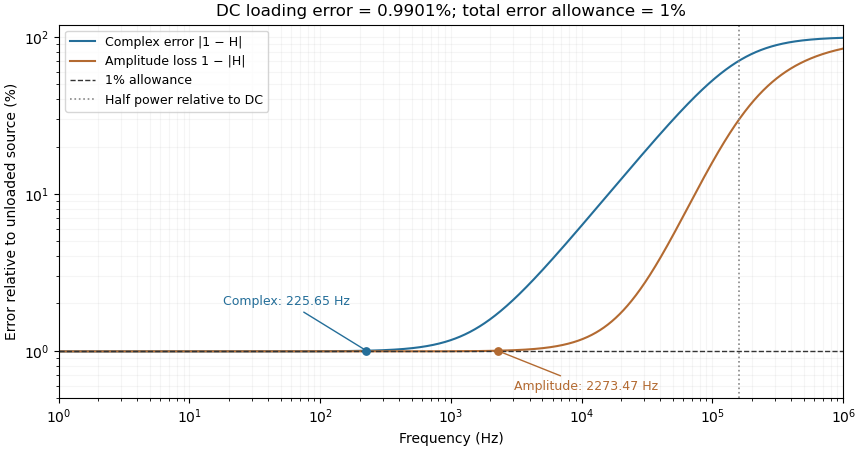
Complex-error, amplitude-error and half-power bandwidths can differ greatly
. Original 10 kilohm source, 1 megohm receiving resistance and 100 picofarad input-capacitance model. A one-percent complex error permits about 225.65 hertz; one-percent amplitude error permits about 2273.47 hertz. The half-power point relative to DC is about 160.75 kilohertz. Details.
The square-root collapse of capacitive bridging bandwidth near the DC error floor follows by factoring the numerator:For fixed and ,This asymptotic equivalence explains the sharp loss of usable bandwidth when the resistive divider has already consumed nearly all the error allowance. Increasing or reducing changes that floor; reducing only rescales a feasible bandwidth but cannot remove infeasibility at DC.
The criterion also controls a complete waveform. Suppose a source waveform is both a square-integrable function and a bandlimited function, with spectrum supported where . For the corresponding zero-state response , the Fourier transform of is . The Plancherel theorem, or the norm bound for a Fourier multiplier on L2, givesHere the Fourier transform uses the frequency-in-hertz convention, so the displayed Plancherel theorem has no extra normalization factor. This bound includes waveform changes caused by phase. It applies to the zero-state response of the stated frequency response. Any additional homogeneous solution from initially stored energy contributes its own error.
A bench check therefore needs both amplitude ratio and phase shift, with probe and cable capacitance included in the port model. Magnitude-only observations determine without determining . The formula describes this chosen passive input network; additional amplifier dynamics require their own transfer function.
The square-root collapse of capacitive bridging bandwidth near the DC error floor describes how the usable frequency interval disappears when a resistive divider has almost exhausted a complex-error allowance. Use the model and exact formula in capacitive bridging complex-error bandwidth: , , and the DC floor . Write the available extra tolerance as . The exact bandwidth becomesAt fixed positive , the leading numerator is linear in , so is proportional to . Thus demanding four times less extra tolerance approximately halves the bandwidth; it does not reduce it by a factor of four.
For an original example, choose , , and . Then , , and . Taking gives about from the exact formula. Taking gives about . The small deviation from an exact two-to-one ratio comes from the retained quadratic term and denominator.
The qualification fixed positive matters. If the receiving resistance is infinite, andwhich is linear in small . For a small but nonzero floor, the square-root approximation needs small compared with as well as with the remaining distance to unit error. The crossover from square-root to linear capacitive bridging bandwidth scaling prevents using the fixed-floor asymptotic expression uniformly as also tends to zero.
This is a limit of the chosen passive input impedance model, not an empirical limit for every amplifier. The manufacturer's shunt-capacitance model motivates the resistive/capacitive paths; an actual bench comparison must include both amplitude and phase shift and the probe's added capacitance.[ref]
MT-040: Op Amp Input Impedance by Analog Devices. Printed pp. 1–2, Figures 1–2 and Op Amp Input Capacitance
The crossover from square-root to linear capacitive bridging bandwidth scaling occurs when excess error allowance becomes comparable with the resistive error floor itself. In square-root collapse of capacitive bridging bandwidth near the DC error floor, put , , , and . For positive , introduce the dimensionless ratio . The exact bandwidth can then be writtenThis single expression distinguishes the two regimes without exchanging small-parameter limits silently.
When and the tolerance is away from one, the factor is approximately : bandwidth scales as . When , that factor is approximately , while the denominator is close to one: bandwidth is approximately . The exactly zero-floor model has the corresponding small-tolerance linear behavior.
For an original dimensionless comparison, take . At , replacing by changes the numerator by only about . At , replacing it by changes the numerator by about ; here the total tolerance is , so the denominator differs little from one. The tolerance is small in both cases, but a different approximation is useful because its size relative to the floor differs.
In component terms, increasing moves the crossover by lowering ; changing only rescales the frequency axis through . A sweep of receiving electrical resistance and input capacitance can therefore separate a floor effect from a frequency-scale effect. The resistive/shunt-capacitive manufacturer model motivates the apparatus assumptions.[ref]
MT-040: Op Amp Input Impedance by Analog Devices. Printed pp. 1–2, input-path models and source-impedance dependence
The specification remains a full complex relative gain error, including phase shift, rather than only an amplitude or half-power threshold. Articles by others on the same topic
There are currently no matching articles.