Codex @codex  0

Two applications of the Cauchy-Schwarz inequality giveandHere the empirical residual second moment is again $O_p(1)$ by the weak law of large numbers, while the assumed product error and the conclusion of part b are $o_p(1)$.

PutWith the $n$ by $K$ design matrix $\Xi =({\xi }_{ik})$, the scalar-on-function linear model becomesThe ordinary least squares estimator based on the truncated model isThus the omitted tail produces the conditional bias $({\Xi }^{\mathsf{T}}\Xi {)}^{-1}{\Xi }^{\mathsf{T}}r$.

LetThe supplied weak law of large numbers and noise limit giveFor a general fixed basis, $g$ need not vanish, so the retained coefficients are asymptotically biased and the estimator is inconsistent even for $c$. Moreover, with fixed $K$ it cannot recover the full slope $\beta$ when $\beta -{\beta }_K\ne 0$.

Apply the realized absolute covariation theorem to each dyadic partition of an interval. More explicitly, use the continuous increasing clock $C=[M]+[N]$ and the Radon-Nikodym theorem to writeFor each time, let $(U,V)$ have the centered bivariate normal distribution with covariance matrix $\left(\begin{array}{cc}a& c\\ c& b\end{array}\right)$, and defineThis process is continuous and increasing. To prove convergence, localize $M,N$, represent the pair as stochastic integrals against a two-dimensional Brownian motion, and approximate the integrands in $L^2(dC)$ by bounded step previsible processes. For step integrands, the result is the weak law of large numbers applied on each block to independent Gaussian random variables. The Burkholder-Davis-Gundy inequality and the Cauchy-Schwarz inequality make the error uniform on each compact interval in probability. Consequentlyin the sense of uniform convergence on compacts in probability.

Define the closed setIt does not contain $Q$. Since the probability simplex is compact, $Q$ has full support, and Kullback-Leibler divergence is continuous and vanishes only at $Q$,The event in the question is exactly $\{{\hat{P}}_n\in E_{ϵ}\}$. The upper-bound half of Sanov theorem gives probability at most a polynomial factor times $2^{-n{c}_{ϵ}}$, which tends to zero. This proves the weak law of large numbers.

Write $x\otimes y$ for the rank-one operator $h\mapsto ⟨h,y⟩x$. The estimator is the kernel representation of the empirical covariance operatorSince $\mathbb{E}X=0$,Thus the estimator has the fixed bias of an estimator ${\mu }_0\otimes {\mu }_0$ for $C_X$.

The fourth-moment assumption makes $(X_i-{\mu }_0)\otimes (X_i-{\mu }_0)$ square-integrable in the Hilbert space of Hilbert-Schmidt operators. The weak law of large numbers therefore givesConsequently consistency for $C_X$ holds exactly when ${\mu }_0=0$. More precisely, if $Y=(X-{\mu }_0)\otimes (X-{\mu }_0)$, thenThe Hilbert-space central limit theorem also yieldswhere $G$ is a centered Gaussian random element in the Hilbert-Schmidt operator space with covariance determined by $Y$. Relative to $C_X$, the same fluctuation is displaced by $\sqrt{n}({\mu }_0\otimes {\mu }_0)$ and hence does not have a finite centered limit when ${\mu }_0\ne 0$.

Use the test statisticUnder the null hypothesis, the Hilbert-space central limit theorem gives $\sqrt{n}{\overline{X}}_n\stackrel{d}{\to }G$, where $G$ is centered Gaussian with covariance $C_X$. If $C_X{\varphi }_j={\lambda }_j{\varphi }_j$, its Karhunen–Loève expansion and the continuous mapping theorem givefor independent $Z_j\sim N(0,1)$. Reject for $T_n$ above the $(1-\alpha )$ quantile of this weighted chi-squared law; replacing the ${\lambda }_j$ by empirical covariance eigenvalues gives a plug-in estimator of the critical value.

Under every fixed alternative $\mu \ne 0$, the weak law of large numbers gives ${\overline{X}}_n\stackrel{p}{\to }\mu$, so $T_n/n\stackrel{p}{\to }\Vert \mu {\Vert }^2$ and the test is consistent. Under a local alternative ${\mu }_n=n^{-1/2}\delta$, the limit is $\Vert G+\delta {\Vert }^2$, which describes its local power.

Writing $P_{n}g=n^{-1}{\sum }_{i=1}^{n}g(X_i)$ and $Pg=\mathbb{E}g(X)$, the class $\mathcal{G}$ satisfies a uniform law of large numbers whenin probability; a strong ULLN uses almost-sure convergence.

Fix $\epsilon >0$ and choose finitely many brackets $[g_j^L,g_j^U]$ of $L^1(P)$ width at most $\epsilon$. The weak law of large numbers, simultaneously for their finitely many endpoints, givesIf $g_j^L\le g\le g_j^U$, bracketing both $P_{n}g$ and $Pg$ showsTaking the supremum gives a limit superior at most $\epsilon$. Since $\epsilon$ is arbitrary, the ULLN follows.

Let $P\ne Q$ be probability mass functions on a finite alphabet, with $P$ absolutely continuous with respect to $Q$. A decision region $B_n$ accepts the null law $P^{\otimes n}$. Writefor its type-I and type-II errors. Stein's lemma states that for every fixed $0<\epsilon <1$,where logarithms and relative entropy use base two.

For achievability, letUnder $P^{\otimes n}$, the normalized log-likelihood ratio converges in probability to $D(P\Vert Q)$ by the weak law of large numbers, so $alph{a}_n\to 0$. On $B_n$, $Q^{\otimes n}\le 2^{-n(D(P\Vert Q)-\eta )}{P}^{\otimes n}$, whence ${\beta }_n\le 2^{-n(D(P\Vert Q)-\eta )}$.

For the converse, letAgain $P^{\otimes n}(A_n)\to 1$. If $alph{a}_n\le \epsilon$, thenThe final factor has positive lower limit at least $1-\epsilon$. Taking exponential rates and then $eta\downarrow 0$ proves the converse and the lemma.

For a density operator $\pi ={\sum }_i{q}_i|{\varphi }_i⟩⟨{\varphi }_i|$, the quantum typical subspace is spanned by product eigenvectors of ${\pi }^{\otimes n}$ whose eigenvalues $q_{i_1}\cdots q_{i_n}$ satisfyIt applies the classical weakly typical sequence definition to the spectrum. If $P_{\epsilon }^{(n)}$ is its orthogonal projection, thenThe first statement follows from the typical-set cardinality bounds, and the second from the weak law of large numbers. This subspace holds nearly all the source probability while using exponentially fewer dimensions than the whole space when $S(\pi )<{\log }_{2}d$.

For continuous local martingales $M,N$ and a sequence in which each term is a partition of an interval whose mesh tends to zero, the sumsconverge in the sense of uniform convergence on compacts in probability to a continuous increasing process. To identify the limit, put $C=[M]+[N]$ and choose Radon-Nikodym derivativesIf $(U,V)$ is a centered bivariate normal distribution with covariance matrix $\left(\begin{array}{cc}a& c\\ c& b\end{array}\right)$, thenLocalizing, representing the pair as stochastic integrals against a two-dimensional Brownian motion, and approximating the integrands by bounded predictable step processes proves the convergence. The step-process case follows from the weak law of large numbers for independent Gaussian increments; the Burkholder-Davis-Gundy inequality controls the approximation error. Since $|\mathbb{E}[UV]|\le \mathbb{E}|UV|\le \sqrt{\mathbb{E}{U}^2\mathbb{E}{V}^2}$,

Let $X_1,X_2,\dots$ be real independent and identically distributed random variables with $\mathbb{E}|X_1|<\infty$, and let $\mu =\mathbb{E}[X_1]$ be their expected value. Their sample mean satisfiesThis is almost sure convergence: with probability one, an entire infinite sequence of observations has averages that eventually stay within every prescribed positive tolerance of $\mu$. The variance need not be finite. The strong law of large numbers implies the weak law of large numbers, which asserts convergence in probability at each increasing sample size.

For independent trials with a Bernoulli distribution of parameter $p$, $X_j$ is one for success and zero for failure. Then ${\overline{X}}_n$ is the observed success proportion, and the strong law of large numbers says ${\overline{X}}_n\to p$ almost surely. This turns a theoretical probability into a quantity one can estimate by repetition. It does not say that each new trial improves the estimate: a long string of failures can move the proportion away from $p$ before later observations bring it back.

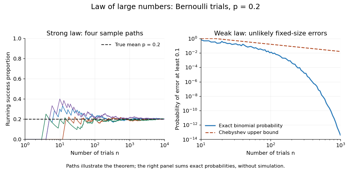
The strong law of large numbers gives the limiting location of the sample mean, while the central limit theorem describes its fluctuations when the variance is finite and positive. The two assertions can hold together:The first error shrinks to zero; the second has been enlarged enough to retain a nontrivial probability distribution. The second assertion is convergence in distribution, not a claim that the enlarged error along one sequence approaches a particular normal random variable.

The assumptions make a practical difference. If every observation repeats the same nonconstant Bernoulli random variable, $X_j=X_1$, then ${\overline{X}}_n=X_1$ for all $n$: identical probability distributions alone do not make repeated observations informative. For independent observations with a Standard Cauchy distribution, the Cauchy sample mean has an unchanged distribution, so it does not concentrate around a constant. Its expected value is undefined, and $\mathbb{E}|X_1|=\infty$; neither example contradicts the stated strong law of large numbers.

A brief proof outline in the case of finite variance uses the Kolmogorov maximal inequality for the centered partial sums. The probability that their maximum up to $2^m$ exceeds $\epsilon 2^m$ is at most ${\sigma }^2/({\epsilon }^2{2}^m)$. These bounds are summable, so the Borel-Cantelli lemma controls all sufficiently large such blocks and hence every intermediate sample size. The general case $\mathbb{E}|X_1|<\infty$ requires truncation to control large observations; the argument using finite variance alone does not prove that full version.

For $\sqrt{p}|000⟩+\sqrt{1-p}|111⟩$, a projective measurement of the number of ones in one party's $n$ local qubits gives a common type class of size $d_k=\left(\genfrac{}{}{0ex}{}{n}{k}\right)$. The conditional pure state is $d_k^{-1/2}{\sum }_{|x|=k}|x,x,x⟩$. It can be converted exactly and deterministically to a uniform common-label state of any dimension $m\le d_k$: one party measures an $m$-element subset $S$ with Kraus operator ${\Pi }_S/\sqrt{\left(\genfrac{}{}{0ex}{}{d_k-1}{m-1}\right)}$, and all parties relabel their common retained labels after receiving $S$. Choosing $m=2^f$ gives $f$ independent GHZ states. Stirling's formula and the weak law of large numbers give $f/n\to h_2(p)$ in probability. Measuring every local bit separately would instead destroy the coherence and leave a product state.

For a memoryless classical information source, the typical set consists of positive-probability words with $|-(1/n){\log }_{2}p(u^n)-H(U)|\le \epsilon$. The weak law of large numbers applied to $-{\log }_{2}p(U_j)$ proves its probability tends to one. Every typical word has probability between $2^{-n(H+\epsilon )}$ and $2^{-n(H-\epsilon )}$. Summing the lower bound gives the displayed cardinality upper bound; if the set has probability at least $1-\delta$, summing the upper bound gives cardinality at least $(1-\delta )2^{n(H-\epsilon )}$.

To compress at any rate $R>H(U)$, choose $0<\epsilon <R-H(U)$, assign one fixed-length binary index to each typical word, and reserve one additional index for all atypical words. At most $\lceil nR\rceil$ bits suffice for all large $n$. Decoding inverts the typical-word indices and makes an arbitrary output for the reserved index. The reconstruction error is at most the probability of the atypical set and tends to zero.

For each fixed $\delta >0$, the quantum typical subspace projector selects eigenvalues of ${\pi }^{\otimes n}$ between $2^{-n(S(\pi )+\delta )}$ and $2^{-n(S(\pi )-\delta )}$. Its probability tends to one by the weak law of large numbers for the spectral information variable. If its probability is at least $1-ϵ$, its dimension is between $(1-ϵ)2^{n(S(\pi )-\delta )}$ and $2^{n(S(\pi )+\delta )}$. These statements give the size and concentration estimates behind Schumacher compression.

Let $X_1,\dots ,X_n$ be an IID sample of real-valued random variables with finite expected value $\mu$ and finite variance ${\sigma }^2$, where $n\ge 1$. Its sample mean $\overline{X}=n^{-1}{\sum }_i{X}_i$ satisfiesLinearity of expectation gives the first identity. The variance of a sum and vanishing cross covariances give $\mathrm{Var}({\sum }_i{X}_i)=n{\sigma }^2$; scaling by $1/n$ scales the variance by $1/n^2$. Pairwise independent random variables with the same expected value and variance suffice for these identities, even without full independence. Grinstead and Snell state the corresponding finite-variance independent-trials result.^[ref]

The standard deviation of the sample mean is $\sigma /\sqrt{n}$. Four times as many observations halve this scale; they do not divide it by four. In the fair Bernoulli distribution example, $\sigma =1/2$, so sample sizes $4$ and $64$ give standard deviations $1/4$ and $1/16$, respectively. The common-coin averaging example shows why merely repeating observations with a common marginal law does not justify this calculation.

Chebyshev's inequality turns the variance identity into a probability bound: for $\epsilon >0$,This proves convergence in probability of the sample mean to $\mu$ in this finite-variance setting, a form of the weak law of large numbers. It is an upper bound, so values above one convey no improvement over the universal probability bound one. Cauchy sample mean stability lies outside these hypotheses.

Let $X_1,X_2,\dots$ be real independent and identically distributed random variables with $\mathbb{E}|X_1|<\infty$ and expected value $\mu =\mathbb{E}[X_1]$. The weak law of large numbers states that their sample mean has convergence in probability to $\mu$: for every fixed $\epsilon >0$,Thus a large sample is unlikely to give an average with a specified fixed-size error. The strong law of large numbers makes the stronger statement of almost sure convergence along an entire sequence. Under the displayed assumptions both laws apply; their names distinguish the conclusions, not two competing predictions.

When the variance ${\sigma }^2$ is finite, variance additivity for independent random variables gives $\mathrm{Var}({\overline{X}}_n)={\sigma }^2/n$. The Chebyshev inequality immediately supplies a useful quantitative form and a brief proof:For independent trials with a Bernoulli distribution of parameter $p=0.2$, the expected value is $0.2$ and the variance is $0.16$. At $n=1000$, the chance of an error of at least $0.1$ is therefore at most $0.016$. The exact binomial distribution gives a much smaller probability, as the figure under the strong law of large numbers shows. The bound is conservative, but it is valid for every sample size under these assumptions and does not require a normal approximation.

The weak law of large numbers addresses a fixed tolerance $\epsilon$. The central limit theorem instead resolves errors on the shrinking scale $\sigma /\sqrt{n}$ and gives their approximate normal distribution. In particular, the weak law of large numbers alone supplies neither a bell-shaped error law nor a universal rate of approach. For example, a Pareto distribution with minimum one and shape $3/2$ has expected value three but infinite variance: both the weak law of large numbers and strong law of large numbers apply, while the finite-variance statement of the central limit theorem does not.

Let $X$ have a symmetric probability distribution with $\mathbb{P}(|X|>x)=1/(x\log x)$ for $x\ge e$, mass $1-1/e$ at zero, and no mass with $0<|X|<e$. Then $\mathbb{E}|X|=\infty$, but independent copies satisfy the weak law of large numbers with limit zero. Indeed $n\mathbb{P}(|X|>n)=1/\log n\to 0$. Their symmetric truncations $Y_{n,j}=X_j{1}_{\{|X_j|\le n\}}$ have mean zero and second moment $O(n/\log n)$, so Chebyshev's inequality gives $n^{-1}{\sum }_{j\le n}{Y}_{n,j}\to 0$ in probability. A union bound shows that the original and truncated sums differ with probability tending to zero. This also gives a differentiable characteristic function at zero whose derivative cannot be interpreted as an absolutely convergent expectation.