Minimize the residual sum of squares $\Vert Y-X\theta {\Vert }^2$. Differentiating gives the normal equations $X^{T}X\hat{\theta }=X^{T}Y$. Full column rank makes $X^{T}X$ positive definite and invertible, so the unique minimizer isSince $\mathbb{E}Y=X\theta$, it is unbiased. The independent common-variance errors give $\mathrm{Cov}(Y)={\sigma }^{2}I$, henceIndependent Gaussian errors with common variance are a sufficient condition for this estimator also to be the maximum likelihood estimator: their log-likelihood differs from $-\Vert Y-X\theta {\Vert }^2/(2{\sigma }^2)$ by terms independent of $\theta$. Profiling an unknown common variance gives the same minimizer. Mean and variance assumptions alone do not specify a likelihood.

For the seven design points, $\bar{x}=0$ and $\overline{x^2}=4$. In increasing time order the design matrix isIts columns are mutually orthogonal: the odd sums vanish and $\sum (x_i^2-4)=0$. Their squared lengths are $7,28,84$, respectively. ThereforeIn particular $\hat{\gamma }={\sum }_i(x_i^2-4)Y_i/84$. Testing for a quadratic contribution means testing $H_0:\gamma =0$ against $\gamma \ne 0$.

The cooling measurements are stated to have zero-mean errors and known common variance, but normality is not explicitly assumed for them. Under the independent-error linear regression model as stated, Chebyshev's inequality gives a valid conservative level-$\delta$ test: reject whenIts null rejection probability is at most $\delta$ because the estimator has mean zero and the calculated variance. If Gaussian errors are additionally assumed, the sharper exact test uses $Z=\sqrt{84}\hat{\gamma }/\sigma \sim N(0,1)$ under the null and rejects for $|Z|>z_{1-\delta /2}$. With only seven observations, exact normal calibration cannot be deduced from the printed moment assumptions alone.

Independence means $\mathrm{Pr}(X\in A,Y\in B)=\mathrm{Pr}(X\in A)\mathrm{Pr}(Y\in B)$ for all Borel sets $A,B$. For variables with a joint density this is equivalent to factorization of that density into the two marginal densities almost everywhere.

The inverse transformation is $x=uv$, $y=(1-u)v$, on $0<u<1$, $v>0$. Its absolute Jacobian determinant is $v$. Multiplying the independent gamma densities by it givesThe density is zero outside that support. Integrating in $v$ with the gamma integral givesIt is a beta density. Its normalization also proves the beta integral ${\int }_0^1{u}^{\alpha -1}(1-u{)}^{\beta -1}du=\Gamma (\alpha )\Gamma (\beta )/\Gamma (\alpha +\beta )$. The joint density consequently factors as this normalized beta density timesThus $V$ is gamma with shape $\alpha +\beta$ and rate $\lambda$, and $U,V$ are independent.

Finally $X=UV$. All relevant first moments are finite, and independence gives $\mathbb{E}X=\mathbb{E}U\mathbb{E}V$, while $\mathbb{E}V=\mathbb{E}X+\mathbb{E}Y>0$. HenceThis identity follows from the particular beta-gamma independence here; a general ratio of random variables would not permit moving expectation through division.

Irrotational motion in this simply connected fluid region has a velocity potential, $u=\nabla \varphi$. Incompressibility gives $\nabla \cdot u=0$, hence $\Delta \varphi =0$.

The moving surface is a material surface: differentiating $y-\eta (x,t)=0$ along a particle gives ${\eta }_t+{\varphi }_x{\eta }_x={\varphi }_y$ at $y=\eta$. Linearizing about a flat stationary surface drops the product term and evaluates at zero, giving ${\eta }_t={\varphi }_y$ there. The Unsteady Bernoulli equation, after dropping quadratic velocity terms and absorbing the time-only constant into $\varphi$, is ${\varphi }_t+p/\rho +gy=0$. The linear capillary pressure at the surface is $p=-T{\eta }_{xx}$ relative to atmosphere, in the sign convention of the source. ThereforeFor $\eta =A\cos (kx-\omega t)$ choose the harmonic potential decaying at infinite depth,Its vertical derivative at zero equals $A\omega \sin (kx-\omega t)={\eta }_t$. Substitution into the dynamic condition gives $-{\omega }^2/k+g+T{k}^2/\rho =0$. ThusThe two positive terms are the gravitational and capillary contributions to the restoring force.

Milne-Thomson's circle theorem inserts an impermeable circular boundary into a two-dimensional irrotational incompressible flow. If $f(z)$ is analytic in a neighborhood of the closed disc and its flow singularities lie outside, the new complex potential outside $|z|=a$ isReflection and coefficient conjugation make the second term analytic outside the circle, with its image singularities inside. On $|z|=a$, $a^2/\bar{z}=z$, so the two terms sum to $2\mathrm{Re}f(z)$: the streamfunction is constant there. Thus no velocity crosses the circle. At infinity the image term tends to the constant $\overline{f(0)}$, which has no effect on velocity, and the far-field flow is retained. This proves the construction, with an additive potential constant immaterial.

Put $A=\mu e^{i\alpha }$, $B=\mu e^{-i\alpha }$. For the dipole the reflected potential is $B/(a^2/z-b)=Bz/(a^2-bz)$, givingIts image pole is $c=a^2/b$, inside the cylinder. The complex velocity isNear $c$, the second term is $C(z-c{)}^{-2}$ with $C=B{a}^2/b^2$, while $v_0(z)=-A/(z-b{)}^2$ is analytic there. The square of the pole term has no residue, nor does $v_0^2$. The cross term has residue $2C{v}_0^{\prime }(c)$, soTake the contour counterclockwise around the cylinder, as in the supplied Blasius force theorem. The residue theorem gives $\frac{1}{2}i\rho \oint (w^{\prime }{)}^{2}dz=-\pi \rho \mathrm{Res}(w^{\prime }{)}^2$. ThereforeThe force points toward the dipole. Its independence of dipole orientation follows from the product $AB={\mu }^2$ in the sole residue contribution.

Set $u=r\psi$, choose $\alpha >0$ for a negative bound-state energy, and write $\kappa =2mK/{\hslash }^2$. Multiplying the radial equation by $r$ givesFor $u=e^{-\alpha r}f$, its second derivative is $e^{-\alpha r}(f^{\prime \prime }-2\alpha f^{\prime }+{\alpha }^{2}f)$. Substitution cancels the two ${\alpha }^2$ terms and givesFor the physical hydrogen problem, the angular eigenvalue has $\ell$ a nonnegative integer. Regularity at the origin selects the Frobenius exponent $u\sim r^{\ell +1}$, rather than the singular branch. PutThe equation for the series factor $v=f/r^{\ell +1}$ is $r{v}^{\prime \prime }+(2\ell +2-2\alpha r)v^{\prime }+(\kappa -2\alpha (\ell +1))v=0$, and coefficient comparison yieldsThe regular confluent-hypergeometric solution generically grows like $e^{2\alpha r}$ in this series factor; after the extracted $e^{-\alpha r}$ it is not normalizable. A bound state requires termination at some degree $q\ge 0$, namely $2\alpha (q+\ell +1)=\kappa$. Thus $n=q+\ell +1$ is an integer greater than $\ell$, andRegularity, normalizability and the integer angular index are the physical conditions selecting this spectrum; the differential equation without those conditions would admit many other solutions.

For $n=1$, necessarily $\ell =0$ and $q=0$. With $a_0={\hslash }^2/(mK)$,A normalized spatial ground state is ${\Psi }_1=(\pi a_0^3{)}^{-1/2}{e}^{-r/a_0}$. In spherical coordinates the radial probability has weight $r^{2}dr$. Constants and the angular integral cancel in the tail ratio. The supplied integral with $\lambda =2/a_0$ gives

Write the position of a mass element relative to the centre of mass as $r$. Expand its squared velocity and integrate:The mixed term vanishes because $\int rdm=0$. Alsousing the scalar triple-product identity. ThereforeIn principal axes the inertia tensor is diagonal, so the second term is $\frac{1}{2}(A{\omega }_1^2+B{\omega }_2^2+C{\omega }_3^2)$. Substituting the three Euler-angle components given in the source gives its displayed kinetic-energy expression directly.

For $A=B$, the first two component squares have opposite mixed terms and sum to ${\dot{\theta }}^2+{\dot{\varphi }}^2{\sin }^2\theta$. Put $n=\dot{\psi }+\dot{\varphi }\cos \theta$. Using the orientation-dependent potential printed in the source therefore gives the formal modelThe cyclic coordinates $x,y,\psi$ have conserved momenta $M\dot{x},M\dot{y},Cn$. Consequently $\dot{x},\dot{y},n$ are constant. The coordinate $\varphi$ is also cyclic, withFor imposed fixed tilt $\theta =\alpha \in (0,\pi /2)$, conservation of $n$ and $p_{\varphi }$ forces $\dot{\varphi }=\Omega$ constant. Impose the fixed-height condition $z=h$ in this formal constrained model. Its $\theta$ equation isSet the tilt constant and divide by its nonzero sine. This givesA real polynomial root requires its quadratic discriminant to be nonnegative:When this condition holds the two algebraic rates are $(Cn\pm \sqrt{C^2{n}^2-4AMgh\cos \alpha })/(2A\cos \alpha )$.

There is a physical inconsistency in the printed data that must be kept distinct from this algebra. If $(x,y,z)$ are literally Cartesian coordinates of the centre of mass in uniform gravity, the gravitational potential is $Mgz$, not $Mgz\cos \theta$. The printed Lagrangian consequently does not follow from that Cartesian-height interpretation. Moreover its unconstrained $z$ equation is $\ddot{z}=-g\cos \theta$, so constant height at the indicated tilt requires a constraint reaction. The requested rate and discriminant follow from the printed orientation-dependent potential with fixed height imposed; a standard heavy-top interpretation instead uses a height proportional to an axis distance times $\cos \theta$, with the reference point and corresponding inertia specified consistently. The kinetic-energy derivation is independent of this source inconsistency.

A sufficient regular-level condition is $\nabla f(x)\ne 0$ at every point with $f(x)=0$. The implicit function theorem then makes the zero level a two-dimensional continuously differentiable submanifold. Its tangent space isFor a minimizing pair $(a,b)$ and any tangent vector $v\in T_a{S}_f$, take a differentiable surface curve $x(s)$ with $x(0)=a$, $x^{\prime }(0)=v$. The function $\Vert x(s)-b{\Vert }^2$ has a minimum at zero, so its derivative $2(a-b)\cdot v$ vanishes. Varying the other point similarly proves orthogonality to $T_b{S}_g$.

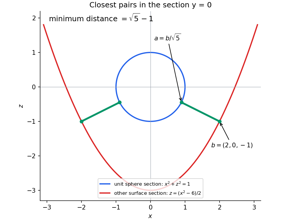
For the particular surfaces, minimize the distance from the origin to the second surface first. Put $u=x^2$, $v=y^2$, so $u,v\ge 0$ and $z=(u-v-6)/2$. ThenLet $s=u-v$. Since $u+v\ge |s|$, this is at least $|s|+(s-6{)}^2/4$, with equality when one of $u,v$ is zero. For $s\ge 0$, this quadratic has its minimum at $s=4$, with value 5. For $s\le 0$, it decreases up to zero and has minimum9 on that half-line. The global minimum is therefore5, attained atAll points of this surface lie outside the unit sphere. For any such $b$, the distance to the sphere is $\Vert b\Vert -1$, attained at $a=b/\Vert b\Vert$ by the triangle inequality. ConsequentlyThis is a global minimization, not merely a stationary-point calculation.

A Hausdorff space separates any two distinct points by disjoint open neighborhoods. For a subspace $A\subseteq X$, intersect such neighborhoods in $X$ with $A$ to obtain disjoint neighborhoods in the subspace topology. Thus subspaces inherit the Hausdorff property.

If $(z_1,z_2)$ lies off the diagonal of a Hausdorff space's square, choose disjoint open neighborhoods $U$ of $z_1$ and $V$ of $z_2$. The open rectangle $U\times V$ contains the pair and avoids the diagonal. Therefore its complement is open and the diagonal is closed.

The map $F:X\times Y\to Z\times Z$ given by $F(x,y)=(f(x),g(y))$ is continuous by the coordinate criterion from E3. The equality locus is $F^{-1}({\Delta }_Z)$ and is closed as an inverse image of a closed set.

Let $q:X\to X/\sim$ be the quotient map. If the quotient is Hausdorff, apply the same argument to $q$ in both coordinates:is closed in $X\times X$.

Conversely suppose $R$ is closed and $q$ is open. Take two distinct quotient points, with representatives $x,y$. Since $(x,y)\notin R$, an open rectangle $U\times V$ around it avoids $R$. The images $q(U)$ and $q(V)$ are open quotient neighborhoods. They are disjoint, because a quotient point in their intersection would have equivalent representatives $u\in U$, $v\in V$, giving $(u,v)\in R$. Hence the quotient is Hausdorff. Thus closedness of the relation and openness of the quotient map suffice for a Hausdorff quotient.

The product topology on $X\times Y$ has the open rectangles $U\times V$, with $U$ open in $X$ and $V$ open in $Y$, as a topological basis. The projection preimages are $p_X^{-1}(U)=U\times Y$ and $p_Y^{-1}(V)=X\times V$, so both projections are continuous.

If $f:Z\to X\times Y$ is continuous, both coordinate compositions are continuous. Conversely, if both are continuous, thenis open for every basic rectangle, proving continuity of $f$. Given paths between two chosen endpoints in each factor, their coordinatewise pair is therefore a continuous path in the product, proving that a product of path-connected spaces is path-connected.

For the compact-neighborhood assertion, fix $x\in K$. For each $y\in L$, choose an open rectangle $U_y\times V_y$ containing $(x,y)$ inside $W$. Compactness of $L$ chooses finitely many $V_{y_j}$ covering $L$. PutThen $x\in U_x$, $L\subseteq V_x$, and $U_x\times V_x\subseteq W$: any point of $V_x$ belongs to one of those rectangles' second factors, while $U_x$ lies in every first factor.

Compactness of $K$ now selects finitely many $U_{x_i}$ covering $K$. SetThese are open, contain $K$ and $L$, and if $(u,v)\in U\times V$, choose an $i$ with $u\in U_{x_i}$ and use $v\in V_{x_i}$. HenceIf $K$ or $L$ is empty, take the corresponding open factor empty and the other factor the whole space; the assertions then hold directly. No Hausdorff assumption on the factors is needed.