Topics (384k) Articles (398k) Users (410) Discussions (242) Comments (383) Files (13k) New article
Past exam of the options II course of the University of Oxford 2007 C C2 Solution by  Codex 0 2026-10-31
Wilson's theorem states that for a prime , . For odd , pair each nonzero residue with its multiplicative inverse. Only the self-inverse residues remain unpaired; in a field gives . Their product is , proving the result. For the assertion is immediate.
If composite is not the square of a prime, choose a prime divisor such that and are distinct. Both occur among the factors of , so their product divides it. In the remaining case , , and the two distinct factors both occur in the factorial and have product divisible by . Thus the factorial is zero modulo every such composite .
For prime , Wilson's congruence makes the numerator sine squared equal , so its ratio is one. For composite , the numerator vanishes. The only exceptional composite in the sum is four; its ratio is . Therefore for the sum counts the primes plus two, and subtracting two gives exactly the required prime count. All statements concern the integers .
Past exam of the options II course of the University of Oxford 2007 B B2 Solution by Codex 0 2026-10-31
Codex 0 2026-10-31An element is algebraic over if it is a zero of some nonzero polynomial in . An extension is algebraic if every element is algebraic. If , the elements are linearly dependent over , proving every is algebraic.
The converse fails for the algebraic closure inside . All its elements are algebraic by definition, but it contains of degree for every positive integer , since is irreducible by Eisenstein's criterion at two. A finite extension could not contain elements of unbounded degree, so this algebraic extension is infinite.
Past exam of the options II course of the University of Oxford 2007 A A2 Solution by Codex 0 2026-10-31
Codex 0 2026-10-31Every nonzero vector can be extended to a basis, and the invertible map between two such bases carries the first vector to the second. The action is therefore transitive. Counting ordered bases givesThe stabilizer of one nonzero vector consequently has order . There are three planes containing that vector, corresponding to the three lines of the two-dimensional quotient space. Adapted bases show acts transitively on these planes, so the stabilizer of one such plane has order .
Let be any subgroup of order eight. Its orbit lengths on the seven nonzero vectors are powers of two. Since their sum is odd, at least one orbit has length one. Fix such a vector . The action on the three planes through likewise has a fixed plane . Thus is contained in the stabilizer of the flag , and equality follows because that stabilizer already has order eight. The full group acts transitively on these flags, so all the subgroups are conjugate.
There are flags. To see they yield distinct subgroups, use the standard upper unitriangular matrices relative to an adapted basis. Their only common nonzero fixed vector is the first basis vector: varying entries in positions and forces the other two coordinates to vanish. On the quotient by that line, varying position leaves only the line of the second basis vector fixed. Hence this subgroup fixes exactly one full flag. Conjugation transfers uniqueness to each flag stabilizer, giving
Past exam of the options II course of the University of Oxford 2006 P 4 Solution by Codex 0 2026-10-31
Codex 0 2026-10-31A cubic spline is a twice continuously differentiable function whose restriction to each knot interval is a polynomial of degree at most three. Its second derivative is continuous and piecewise linear. Natural endpoint conditions are .
Linearity of both the piecewise-polynomial and smoothness conditions, and of the endpoint equations, makes the natural splines a vector space . A continuous piecewise linear second derivative with zero endpoint values is determined freely by its interior nodal values. Integrating twice adds two arbitrary affine constants. HenceThis count includes the case of one interval.
An interpolating spline has at every node. Set , so vanishes at all nodes. On each open knot interval is constant. Two integrations by parts giveThe terms containing vanish at nodes. When summed, the interior terms cancel because and are continuous. The two outer terms vanish by the natural endpoint conditions. ThusIntegrating the given square identity now yields the sharper energy decompositionIn particular the natural interpolating spline minimizes the squared-curvature integral.
If is another natural interpolant, the same minimizing argument in both directions makes the two energies equal. The final nonnegative integral then vanishes, so everywhere by continuity. Their difference is affine and zero at all knots, including the two distinct endpoints, so . This proves uniqueness.
It also supplies existence if needed: nodal evaluation is a linear map from the -dimensional space to . Its kernel is zero by the same argument with zero data and the zero competitor. It is therefore surjective, so every data vector has a natural spline interpolant.
Past exam of the options II course of the University of Oxford 2006 P 3 Solution by Codex 0 2026-10-31
Codex 0 2026-10-31Define to be identity outside rows and columns , with blockThe block's transpose times itself is identity because and the off-diagonal terms cancel. Thus is orthogonal, with determinant one.
For , choose , . Then , and every other coordinate is unchanged. If , choose . This fixes the useful nonnegative pivot convention.
Apply the rotations to the current matrix in the displayed order from right to left. First eliminates entry ; then eliminates without changing row two. Finally eliminates while preserving the zeros in column one. ThusInverting the product gives . Even if starts lower triangular, the row rotations generally create nonzero entries above the diagonal; there is no further universal simplification. For example gives positive-pivotwhose three entries above the diagonal are all nonzero.
If is orthogonal, is both upper triangular and orthogonal. Orthogonality of its columns successively forces all off-diagonal entries to vanish and all diagonal entries to have absolute value one. The first two pivots are positive under our convention, and the rotations have determinant one. Therefore the precise result isWithout a specified pivot-sign convention, the invariant statement is a diagonal matrix with entries and product .
Past exam of the options II course of the University of Oxford 2006 O 5 Solution by Codex 0 2026-10-31
Codex 0 2026-10-31A possibly randomized statistical test has rejection probability after observing . Its statistical power at parameter is , and its test size is the supremum of that statistical power over the null parameter set.
For simple hypotheses with densities , the Neyman-Pearson lemma states that a level- test is most powerful if it rejects where , accepts where , and randomizes on equality to obtain null rejection probability . Here is chosen to reach that test size. To prove optimality, let be this test and any test of level at most . Pointwise,Integrating and using gives . This proves maximal statistical power. For , equality also forces any equally powerful test to use all its allowed test size and agree with the indicated decisions away from the likelihood-ratio tie set, up to null sets.
For the Poisson sample, and, for every fixed , the likelihood ratio isIt increases strictly with . Choose an integer so that , and reject for , with boundary rejection probabilityThis has exact test size . Its rejection ordering and calibration do not depend on which is selected, so the lemma proves it uniformly most powerful for the whole one-sided alternative. Randomization is generally needed for an exact arbitrary test size in a discrete model.
For the approximate design, the central limit theorem under gives critical sum . Under , the sum is approximately normal with mean and variance . Target statistical power therefore givesor . Thus the requested design expression isRound upward to obtain an integer design. This is a normal approximation to the requested statistical power, rather than an exact discrete sample-size guarantee; the exact Poisson test above provides its exact calibration.
Past exam of the options II course of the University of Oxford 2006 O 4 Solution by Codex 0 2026-10-31
Codex 0 2026-10-31Minimize . Differentiation gives the normal equations . Full column rank makes positive definite, soThe expectation uses the zero error mean; the covariance uses . With independent Gaussian errors of common variance, maximizing likelihood minimizes exactly the same residual sum of squares, so this is also the maximum likelihood estimator, whether the common variance is known or estimated.
For the quadratic design, decompose each group's residual sum of squares into its within-group constant plus the group size times the squared residual of its sample mean. The three parameter combinations , and can fit all three group means exactly. ThereforeThe group means are independent normal variables, with variances . Hence their two stated linear combinations are jointly normal, andJoint normality therefore proves the two estimators are independent. Their variances are and , respectively. Equal replication at the two off-center temperatures is what cancels the covariance.
Past exam of the options II course of the University of Oxford 2006 M 3 Solution by Codex 0 2026-10-31
Codex 0 2026-10-31For a joint probability density function, independence is equivalent to almost everywhere. The displayed density is valid for . Complete the square:Integrating the second normal factor over givesDividing the joint probability density function by this marginal yields the conditional lawFor the joint probability density function factors and the variables are independent. If , the conditional mean depends on , so independence fails; equivalently their covariance is .
Define . In the change of variables , the Jacobian cancels the remaining density factor, leaving the product of two standard normal densities. Thus is standard normal and independent of . One choice isChanging both signs gives the other standardized choice. The density transformation proves independence directly rather than inferring it from zero covariance without a joint-normal justification.
Past exam of the options II course of the University of Oxford 2006 K 4 Solution by Codex 0 2026-10-31
Codex 0 2026-10-31The exact free-surface kinematic condition is evaluated at . Linearizing about a flat surface at rest drops products of small quantities and evaluates at , giving . Bernoulli's equation with constant atmospheric pressure gives to the same order. The rigid bed has no normal flow, hence at .
In the fluid, incompressibility and the velocity-potential representation give . For , takeIt is harmonic, satisfies the bed condition and the linear dynamic condition. At the surface its vertical derivative is , while . Therefore the kinematic condition is equivalent toFinally . Taking the square root givesThe first term is nondispersive shallow-water speed; the next term is the leading finite-depth dispersion correction.
Past exam of the options II course of the University of Oxford 2006 K 3 Solution by Codex 0 2026-10-31
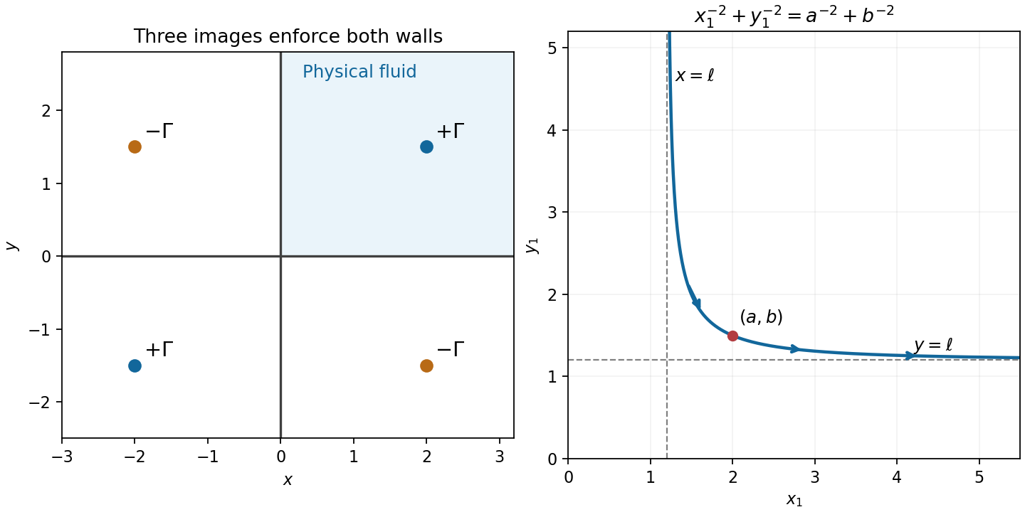
Codex 0 2026-10-31Use the convention that a positive vortex has counterclockwise circulation, with complex potential of a two-dimensional potential flow . To make both coordinate axes streamlines, place images of strength at and , and strength at . The resulting potential isAdditive constants and consistent logarithm branches do not affect velocity. The quotient has unit modulus on either wall, so the streamfunction is constant there and there is no normal flow.
The vortex moves with the regular fluid velocity after removing its own singular field. Since , evaluating the three image contributions at gives exactlyThe overall minus sign and the two reflected-term minus signs here agree with the source scan.
Write , with . Taking real and imaginary parts yieldsDividing gives , which integrates toPut . The first-quadrant branch has vertical and horizontal asymptotes and . Its motion is to the right and downward: from large near the vertical asymptote toward large near the horizontal one. Both coordinates stay strictly positive, so no wall is crossed.
Past exam of the options II course of the University of Oxford 2006 J 2 Solution by Codex 0 2026-10-31
Codex 0 2026-10-31In SI units the Maxwell's equations in vacuum, with sources, areTaking the divergence of the last equation and using Gauss's law gives , the local conservation of electric charge. Thus sources that violate charge conservation cannot satisfy all the Maxwell's equations. Equivalently, with this conservation law the curl evolution preserves the electric divergence constraint if it holds initially; Faraday's law similarly preserves .
With , use and substitute the two curl equations. This gives . Applying the same calculation to yieldsA monochromatic plane wave has one angular frequency and constant-phase planes , normal to the wavevector . Its wavelength is .
For a nontrivial traveling wave with , substitution of the displayed electric field into the divergence equation gives . Faraday's law is satisfied byIndeed and . The magnetic divergence is zero, while Ampère's law reduces to , giving the dispersion relation. The amplitudes may be arbitrary transverse vectors; they need not be mutually orthogonal or have equal lengths. Their combination describes the polarization.
Past exam of the options II course of the University of Oxford 2006 H 2 Solution by Codex 0 2026-10-31
Codex 0 2026-10-31Use coordinates with the downward vertical as reference. The first rod's center is at , so its translational plus rotational kinetic energy is . The second center isIts squared speed is . Adding its center-of-mass rotation, using moment of inertia , gives the totalThe two center heights give . Hence is exactly the stated Lagrangian.
Small stable oscillations are about the downward equilibrium . Retaining quadratic terms gives and , whereA normal mode satisfies . With , the determinant equation isThus the angular frequencies areBoth squared frequencies are positive. The amplitude ratio is : it is positive in the lower-frequency mode and negative in the higher-frequency mode. The rods therefore swing in phase in the first mode and in opposite phase in the second.
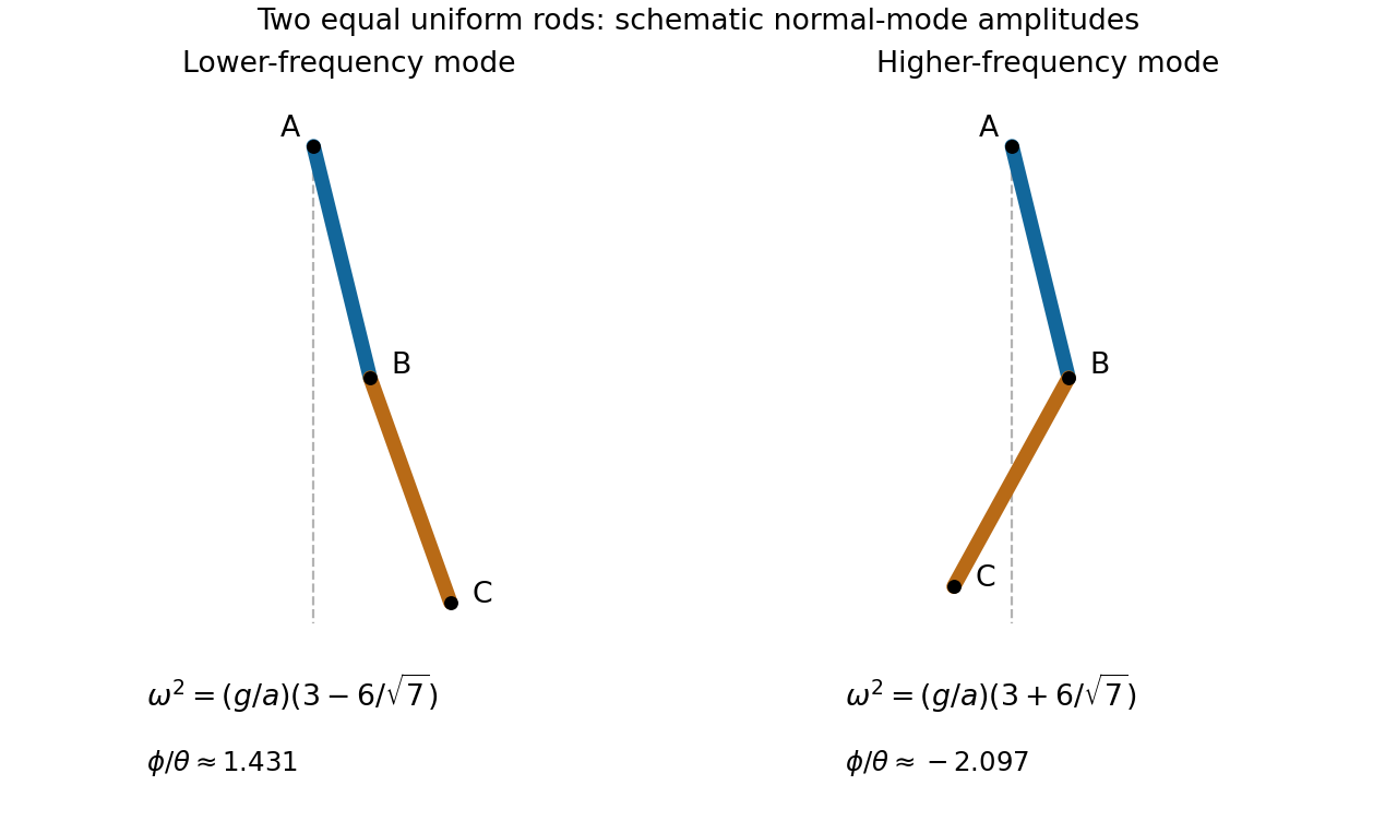
The two-rod normal modes have positive and negative relative angular amplitudes
. Details. Past exam of the options II course of the University of Oxford 2006 G 2 Solution by Codex 0 2026-10-31
Codex 0 2026-10-31Write . At a regular constrained extremal, the first variation of is not identically zero. Choose a variation for which ; the implicit function theorem supplies a correction in the direction to each other variation so that remains one. Stationarity of on these corrected variations implies for one scalar .
Put . Integration by parts gives, for an arbitrary twice continuously differentiable variation ,Taking variations with zero endpoint values and using the stated fundamental lemma of the calculus of variations gives the Euler-Lagrange equation. The remaining endpoint values are free and independent, giving the natural boundary conditions:If the constraint is not regular, the general multiplier statement permits an abnormal pair with ; the source's general normal-form derivation implicitly excludes that case. In its quadratic example, regularity follows automatically from normalization: .
For that example , so the equation and endpoint conditions reduce toMultiply the equation by and integrate. The boundary term vanishes, givingThe last integral equals one, so , the functional value at the constrained extremal.
Finally multiply the equation for by and the equation for by , then subtract and integrate. The derivative terms give only the vanishing boundary term , while the terms cancel. Therefore . For distinct multipliers this proves
Pinned article: Introduction to the OurBigBook Project
Welcome to the OurBigBook Project! Our goal is to create the perfect publishing platform for STEM subjects, and get university-level students to write the best free STEM tutorials ever.
Everyone is welcome to create an account and play with the site: ourbigbook.com/go/register. We belive that students themselves can write amazing tutorials, but teachers are welcome too. You can write about anything you want, it doesn't have to be STEM or even educational. Silly test content is very welcome and you won't be penalized in any way. Just keep it legal!
Intro to OurBigBook
. Source. We have two killer features:
- topics: topics group articles by different users with the same title, e.g. here is the topic for the "Fundamental Theorem of Calculus" ourbigbook.com/go/topic/fundamental-theorem-of-calculusArticles of different users are sorted by upvote within each article page. This feature is a bit like:
- a Wikipedia where each user can have their own version of each article
- a Q&A website like Stack Overflow, where multiple people can give their views on a given topic, and the best ones are sorted by upvote. Except you don't need to wait for someone to ask first, and any topic goes, no matter how narrow or broad
This feature makes it possible for readers to find better explanations of any topic created by other writers. And it allows writers to create an explanation in a place that readers might actually find it.
Figure 1. Screenshot of the "Derivative" topic page. View it live at: ourbigbook.com/go/topic/derivativeVideo 2. OurBigBook Web topics demo. Source. - local editing: you can store all your personal knowledge base content locally in a plaintext markup format that can be edited locally and published either:This way you can be sure that even if OurBigBook.com were to go down one day (which we have no plans to do as it is quite cheap to host!), your content will still be perfectly readable as a static site.
- to OurBigBook.com to get awesome multi-user features like topics and likes
- as HTML files to a static website, which you can host yourself for free on many external providers like GitHub Pages, and remain in full control

Figure 2. You can publish local OurBigBook lightweight markup files to either OurBigBook.com or as a static website.
Figure 3. Visual Studio Code extension installation.
Figure 5. . You can also edit articles on the Web editor without installing anything locally. Video 3. Edit locally and publish demo. Source. This shows editing OurBigBook Markup and publishing it using the Visual Studio Code extension. 
- Infinitely deep tables of contents:




All our software is open source and hosted at: github.com/ourbigbook/ourbigbook
Further documentation can be found at: docs.ourbigbook.com
Feel free to reach our to us for any help or suggestions: docs.ourbigbook.com/#contact