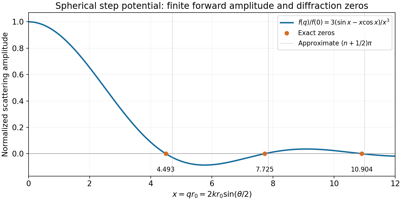
Apart from the finite forward limit, amplitude zeros obey $\sin x-x\cos x=0$, or $\tan x=x$, where $x=q{r}_0$. The first positive root is $x_1\simeq 4.49341$. Since the accessible range is $0\le x\le 2k{r}_0$,Thus there are no zeros for $k<k_c$; the first enters at the largest momentum transfer, $\theta =\pi$, when $k=k_c$.

For larger roots, $x_n$ lies just below $a_n=\pi (n+\frac{1}{2})$, $n=1,2,\dots$. Expanding $\tan (a_n-\epsilon )\simeq 1/\epsilon$ gives $x_n=a_n-1/a_n+O(a_n^{-3})$. Keeping its leading term yields the requested diffraction estimateExactly, replace the numerator $\pi (n+\frac{1}{2})$ by the corresponding root $x_n$. The displayed approximation is a large-$q{r}_0$ root approximation: taking $k$ large at fixed low order does not make $x_1$ equal to $3\pi /2$. For example, the exact first angle at high $k$ is approximately $4.49341/(k{r}_0)$, not $4.71239/(k{r}_0)$.

The spherical potential has a rotationally symmetric Fourier transform, so choose the polar axis of the integration along $\mathbf{q}$. With $q=|{\mathbf{k}}_f-{\mathbf{k}}_i|=2k\sin (\theta /2)$,The first Born approximation therefore givesThere is no azimuthal dependence. At $q=0$, the bracket is $(q{r}_0{)}^3/3+O(q^5)$, so $f_k(0)=-2m{V}_0{r}_0^3/(3{\hslash }^2)$ is finite, not zero. The approximation assumes scattering weak enough for the incident plane wave to replace the distorted wave inside the interaction integral.

Far from a short-range potential, the particle is locally free. The imposed incoming boundary condition is a unit-amplitude plane wave travelling along $+z$, while an outgoing free spherical wave has radial dependence $e^{ikr}/r$. The scattering coefficient can depend on direction, givingFor the Schrödinger probability current, $\mathbf{j}=(\hslash /m)\mathrm{Im}({\psi }^{\ast }\nabla \psi )$, the incident flux is $j_{\mathrm{in}}=\hslash k/m$. The outgoing scattered radial flux, separated from the incident beam, is $j_{\mathrm{sc},\mathrm{r}}\sim (\hslash k/m)|f_k{|}^2/r^2$. Thus the outgoing rate through $r^{2}d\Omega$, divided by incident flux, givesThis elastic-scattering result uses the same incoming and outgoing wavenumber and the usual outgoing-wave boundary condition.

With $A^{\mu }=(0,\mathbf{A})$, the lowered components are $A_{\mu }=(0,-\mathbf{A})$. Define $\mathbf{\pi }=-i\nabla +e\mathbf{A}$ and $\mathbf{B}=\nabla \times \mathbf{A}$. This convention describes physical charge $q=-e$. Since $F_{ij}=-{ϵ}_{ijk}{B}_k$,Writing $\psi =e^{-i(m+E)t}\varphi$ makes the squared equationDrop $E^2$ relative to $2mE$ and write $\varphi =(\phi ,\chi {)}^T$. Both two-component blocks obey the Pauli equationThe gauge-covariant kinetic term contains ${\mathbf{p}}^2/(2m)$, $e(\mathbf{A}\cdot \mathbf{p}+\mathbf{p}\cdot \mathbf{A})/(2m)$, and $e^2{A}^2/(2m)$: free kinetic, orbital magnetic, and diamagnetic contributions. The spin term is $-\mathbf{\mu }\cdot \mathbf{B}$ with $\mathbf{\mu }=-e\mathbf{\sigma }/(2m)$, giving spin gyromagnetic factor $g=2$ at this order. In uniform $\mathbf{B}$ and symmetric gauge, the orbital term is $e\mathbf{B}\cdot \mathbf{L}/(2m)$.

Squaring introduces extra formal solutions unless the original first-order equation is retained. In the usual positive-energy Dirac basis it relates the small lower component to the upper one by $\chi =(\mathbf{\sigma }\cdot \mathbf{\pi })\phi /(2m+E)\simeq (\mathbf{\sigma }\cdot \mathbf{\pi })\phi /(2m)$. Thus these are not two independent nonrelativistic particles. Restoring units places $\hslash$ in the spin term, $e\hslash \mathbf{\sigma }\cdot \mathbf{B}/(2m)$.

Use $F_{\mu \nu }={\partial }_{\mu }{A}_{\nu }-{\partial }_{\nu }{A}_{\mu }$. The stated derivative convention gives $[D_{\mu },D_{\nu }]=-ie{F}_{\mu \nu }$. Also $[{\gamma }^{\mu },{\gamma }^{\nu }]=-2i{\sigma }^{\mu \nu }$. Splitting products into symmetric and antisymmetric parts therefore yieldsMultiplying the first-order equation by $i{\gamma }^{\mu }{D}_{\mu }+m$ now givesThe antisymmetric derivative commutator is the electromagnetic field strength. It is the extra term absent when squaring an uncoupled Dirac operator with commuting derivatives, and it generates the spin–magnetic-field interaction in the nonrelativistic limit.

Let $U(x)=e^{ie\alpha (x)}$, ${\psi }^{\prime }=U\psi$, and $A_{\mu }^{\prime }=A_{\mu }+{\partial }_{\mu }\alpha$. Direct differentiation in the gauge covariant derivative givesThe gradient of the local phase is exactly cancelled by the potential transformation. Since $U$ is scalar in spinor space and commutes with the Dirac matrices,Consequently a solution is mapped into a solution: the minimally coupled Dirac equation is covariant under the local U(1) gauge symmetry. The operator and wavefunction both transform; ordinary differentiation of the transformed wavefunction alone would leave an extra phase-gradient term.

Work with $\eta =\mathrm{diag}(1,-1,-1,-1)$ and $/\partial ={\gamma }^{\mu }{\partial }_{\mu }$. Multiplying the free Dirac equation by the operator with the opposite mass sign givesThe ordinary derivatives commute, so only the symmetric part of ${\gamma }^{\mu }{\gamma }^{\nu }$ contributes. Requiring this operator to factor the Klein-Gordon equation, $({\partial }^{\mu }{\partial }_{\mu }+m^2)\psi =0$, for arbitrary free momenta givesThus the Dirac matrices represent the corresponding Clifford algebra. The inference uses factorization for the general free equation; the fact that one specially chosen wavefunction happens to solve both equations would not alone determine every matrix anticommutator.

Low excited states lie many thermal energies above the ground state at the inferred temperature, so their contributions to the atomic internal partition function are exponentially suppressed. For hydrogen, $E_2-E_1=10.2$ eV and the level degeneracy ratio is $g_2/g_1=4$. HenceThe ground-state approximation is therefore excellent for this level under the assumed thermal-equilibrium conditions. A formal sum over infinitely many isolated-atom Rydberg states needs a physical high-level cutoff in a plasma; it should not be used to overturn the finite-level Boltzmann estimate. Radiation-driven nonequilibrium populations would require a different model.

Define fractional ionization as $x=n_p/(n_H+n_p)$ and use electrical neutrality. For $x=0.01$ and $n_e=10^9{\mathrm{m}}^{-3}$, $n_H=(1-x)n_e/x=99n_e$. Thus the density form of the Saha equation requiresSolving this monotone equation, conveniently after taking its logarithm, givesThe thermal energy is only about $2.2\%$ of the $13.6$ eV ionization energy. Ionization is not decided by setting $k_{\mathrm{B}}T=R$: the high-energy tail and the large translational state-count factor in chemical equilibrium allow a residual ionized fraction at a much lower temperature. This is the equilibrium estimate for the stipulated density and fraction, without inferring an expansion age from it.

Assume a dilute nondegenerate ideal mixture in thermal and chemical equilibrium, electrical neutrality $N_e=N_p$, and ground-state hydrogen only. Choose the zero of internal energy as a separated proton and electron, so the atom has energy $-R$. Its single-particle partition function contains $e^{R/(k_{\mathrm{B}}T)}$:Their ratio has one remaining power of $V$. Neglecting binding mass in $m_H\simeq m_p$ makes the translational mass factor $(m_e{m}_p/m_H{)}^{3/2}\simeq m_e^{3/2}$. For unresolved ground-state spin states, $g_e{g}_p/g_H=1$: including proton spin gives $2\times 2/4$, or omitting it consistently gives $2\times 1/2$. The given law of mass action therefore yieldsThis is the Saha equation with the degeneracy convention used by the source. Equivalently $n_e^2/n_H=(2\pi m_e{k}_{\mathrm{B}}T/h^2{)}^{3/2}{e}^{-R/(k_{\mathrm{B}}T)}$.

Using the replacement prescribed in the question, $k_{\mathrm{B}}T\to E_F$, givesThe number of electrons in a Debye sphere is consequentlyA useful check eliminates $n_e$: with $r=\hslash {\omega }_{\mathrm{pe}}/E_F$ and $k_F=(3{\pi }^2{n}_e{)}^{1/3}$, $k_F{\lambda }_D=\sqrt{2}/r$ and $N_D=8\sqrt{2}/(9\pi r^3)$.

Having substantially fewer than one electron in this sphere shows that the classical many-particle Debye-screening picture is not applicable. It does not exclude collective plasmons in a degenerate electron gas. A proper zero-temperature Thomas-Fermi screening calculation uses $\partial n/\partial \mu =3n/(2E_F)$ and gives ${\lambda }_{\mathrm{TF}}^2=2{ϵ}_0{E}_F/(3n_e{e}^2)$, rather than literally replacing $T$ by $T_F$. The boxed count follows the source's stated prescription and exposes its physical limitation.

For a nonrelativistic, three-dimensional ideal electron gas with spin degeneracy two,Dividing givesWrite the density-independent coefficient as $K$. From $\hslash {\omega }_{\mathrm{pe}}/E_F=1.384$, $n_e=(K/1.384{)}^6$. In this free-electron model,The result uses the stipulated energy ratio, rather than substituting a separately tabulated aluminium density or plasmon energy.

The Debye length is the distance over which a small, slowly varying electrostatic potential is screened by mobile thermal charges. For classical electrons in a weak potential $\varphi$, their Boltzmann distribution givesTake fixed singly charged ions of density $n_0$. Then $\rho =e(n_0-n_e)\simeq -n_0{e}^2\varphi /(k_{\mathrm{B}}T)$, and Poisson's equation outside a test charge becomes ${\nabla }^2\varphi =\varphi /{\lambda }_D^2$, withThe screened point-charge potential is proportional to $e^{-r/{\lambda }_D}/r$. The derivation assumes nondegenerate statistics and $|e\varphi |\ll k_{\mathrm{B}}T$. Mobile ions would add their own contribution to ${\lambda }_D^{-2}$; the expression here is the electron screening length.

Treat the ions as a stationary neutralizing background and displace the cold electrons by a small longitudinal distance $\xi$. Their electric polarization is $P=-n_{e}e\xi$, so the restoring electric field is $E=-P/{ϵ}_0=n_{e}e\xi /{ϵ}_0$. The electron equation of motion isFor $E=E_0\cos {\omega }_{\mathrm{pe}}t$, the oscillatory velocity is $v=-e{E}_0\sin {\omega }_{\mathrm{pe}}t/(m_e{\omega }_{\mathrm{pe}})$. HenceThe longitudinal mode exchanges electron kinetic energy and electrostatic field energy like a harmonic oscillator, whose mean kinetic and potential energies are equal over a cycle. This is a time-average statement for the coherent oscillation, not thermal equipartition with $k_{\mathrm{B}}T$.

Use $k_{\mathrm{B}}{T}_p=1000$ eV and $k_{\mathrm{B}}{T}_b=100$ eV. The nonrelativistic beam speed and cross-sectional area areHere $V/{\sigma }_p=\sqrt{20}$, ${\sigma }_b^2/{\sigma }_p^2=0.1$, and the exponential in the requested threshold is $e^{-10}$. With $C=\sqrt{e}$,Converting beam density to the magnitude of its electric current givesThis is an order-of-magnitude estimate from the source's asymptotic formula. The numerical hierarchy is only moderate: $V{\sigma }_b/{\sigma }_p^2=\sqrt{2}$. Retaining the background slope at $V-{\sigma }_b$ instead gives about $9.1\times 10^4$ A as a sufficient positive-slope current at that chosen velocity. The difference quantifies the sensitivity of the exponential-tail approximation; an exact kinetic instability threshold requires the dispersion relation. The requested estimate is therefore on the scale of tens of kiloamperes, rather than a precisely determined current.

At $v_{\ast }=V-{\sigma }_b$, the beam's positive slope is $n_b{e}^{-1/2}/(\sqrt{2\pi }{\sigma }_b^2)$, while the background slope has magnitude $n_p{v}_{\ast }{e}^{-v_{\ast }^2/(2{\sigma }_p^2)}/(\sqrt{2\pi }{\sigma }_p^3)$. Thus a nonnegative total slope at this velocity requiresApproximating the background slope by its value at $V$ yieldsEquality is the local marginal-slope condition; strict inequality gives positive resonant drive in this approximation. The numerical $C$ is of order unity and can change when the resonant velocity is optimized or the full wave dispersion is retained.

Replacing $v_{\ast }$ by $V$ in the exponential is controlled only if $V{\sigma }_b/{\sigma }_p^2\ll 1$, in addition to ${\sigma }_b\ll {\sigma }_p$. The two width inequalities alone do not guarantee that extra condition far out on a Maxwellian tail. The preceding unapproximated slope inequality remains available when it is not satisfied.

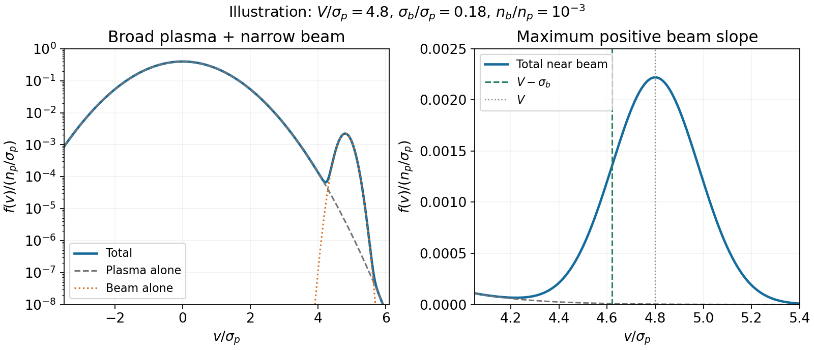
For the shifted beam Maxwell-Boltzmann distribution,On the rising flank put $u=(V-v)/{\sigma }_b>0$. The positive slope is proportional to $u{e}^{-u^2/2}$, whose derivative is $(1-u^2)e^{-u^2/2}$. Its unique positive maximum is at $u=1$, givingThis is the region where beam drive can most readily overcome the negative plasma slope when that background changes little over the narrow beam width. It is an estimate for the first resonant unstable wave, not a proof that every beam-plasma dispersion relation has its exact marginal phase velocity at this value. Both the total slope and the real dispersion relation determine the exact marginal mode.

Define the one-dimensional thermal widths ${\sigma }_p=\sqrt{k_{\mathrm{B}}{T}_p/m_e}$ and ${\sigma }_b=\sqrt{k_{\mathrm{B}}{T}_b/m_e}$. Normalize each velocity distribution to its electron number density:The total is $f=f_p+f_b$. It consists of a broad peak centred at zero and a much narrower displaced beam near $V$, with $V\gg {\sigma }_p\gg {\sigma }_b$. Their areas, rather than their peak heights, are $n_p$ and $n_b$. A weak narrow beam can make a positive-slope region on its low-velocity side even while contributing little to the total density.

Landau damping is the collisionless decay of a plasma wave through resonant energy exchange with particles whose velocity is close to the wave's phase velocity $v_{\varphi }=\omega /k$. Particles slightly slower than the wave tend to gain energy from it; particles slightly faster can give energy to it. For the decreasing resonant part of a Maxwell-Boltzmann distribution, the net transfer is from the wave to the electrons, so the wave amplitude decays.

In the linear Vlasov equation description this is collisionless phase mixing, not a requirement for frequent particle collisions. Fine-scale structure develops in the velocity dependence of the perturbation even while the macroscopic electric field decreases. The resonant contribution to the growth rate has the sign of $\partial f/\partial v$ at a positive wave phase velocity: a negative slope produces damping, whereas a sufficiently positive slope can drive an instability. A population comparison must be local to the resonance; merely counting all particles faster and slower than the wave is not the criterion.

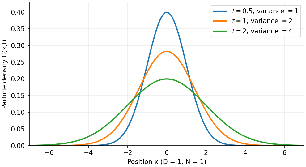
For constant $D$ and no drift, particle conservation and Fick's first law give the one-dimensional diffusion equation ${\partial }_{t}C=D{\partial }_x^{2}C$. For $C=A{t}^{-1/2}{e}^{-x^2/(4Dt)}$,so direct substitution verifies the equation for $t>0$. The Gaussian integral fixes the normalization:This is the heat kernel for a point release, with $C(x,0)=N\delta (x)$ in the distributional limit. It remains centered at zero while its width grows as $t^{1/2}$ and its peak falls as $t^{-1/2}$. To compute the second moment, set $y=x/\sqrt{4Dt}$:using $\int y^2{e}^{-y^2}dy=\sqrt{\pi }/2$ over the whole real line, obtained by integration by parts.

If the mean number of independent unbiased jumps in time $t$ is $⟨m⟩=ft$, conditioning on $m$ gives $⟨x^2(t)⟩=\Delta ⟨m⟩=f\Delta t$. Matching it to the continuum diffusion result yieldsFor fixed-magnitude steps $a$, $\Delta =a^2$. The equality of second moments also holds for Poisson jump times independent of the increments; a Gaussian continuum approximation additionally requires many steps and finite step variance.