Let $C(x)$ be the particle number density, $U(x)$ the conservative potential energy and $F=-dU/dx$ the applied force. In the overdamped regime a viscous drag coefficient $\zeta$ gives drift velocity $v_d=F/\zeta$. Combining this drift with Fick's first law gives the number fluxAt thermal equilibrium, the Boltzmann distribution is $C_{\mathrm{eq}}\propto e^{-U/(k_{\mathrm{B}}T)}$, so $d{C}_{\mathrm{eq}}/dx=F{C}_{\mathrm{eq}}/(k_{\mathrm{B}}T)$. Setting its net flux to zero yieldsThis is the Einstein diffusion relation. The derivation assumes a dilute equilibrium suspension, uniform temperature, linear drift response and a well-defined long-time diffusion coefficient. With a nonzero conservative force, the full transport equation includes drift; the force-free equation in the next section describes spreading without that drift.

Write the one-dimensional random walk endpoint as $x_m={\sum }_{j=1}^m{\xi }_j$, starting at the origin. Assume unbiased, independent increments, each with $⟨{\xi }_j⟩=0$ and $⟨{\xi }_j^2⟩=\Delta$. Expanding the square givesIndependence makes each cross expectation $⟨{\xi }_i⟩⟨{\xi }_j⟩=0$. ConsequentlyUncorrelated increments with the same second moments would suffice. Unbiasedness alone does not remove correlations: persistent or anticorrelated steps need not satisfy this result. The symbol $\Delta$ is already the mean-square step size, with units of length squared.

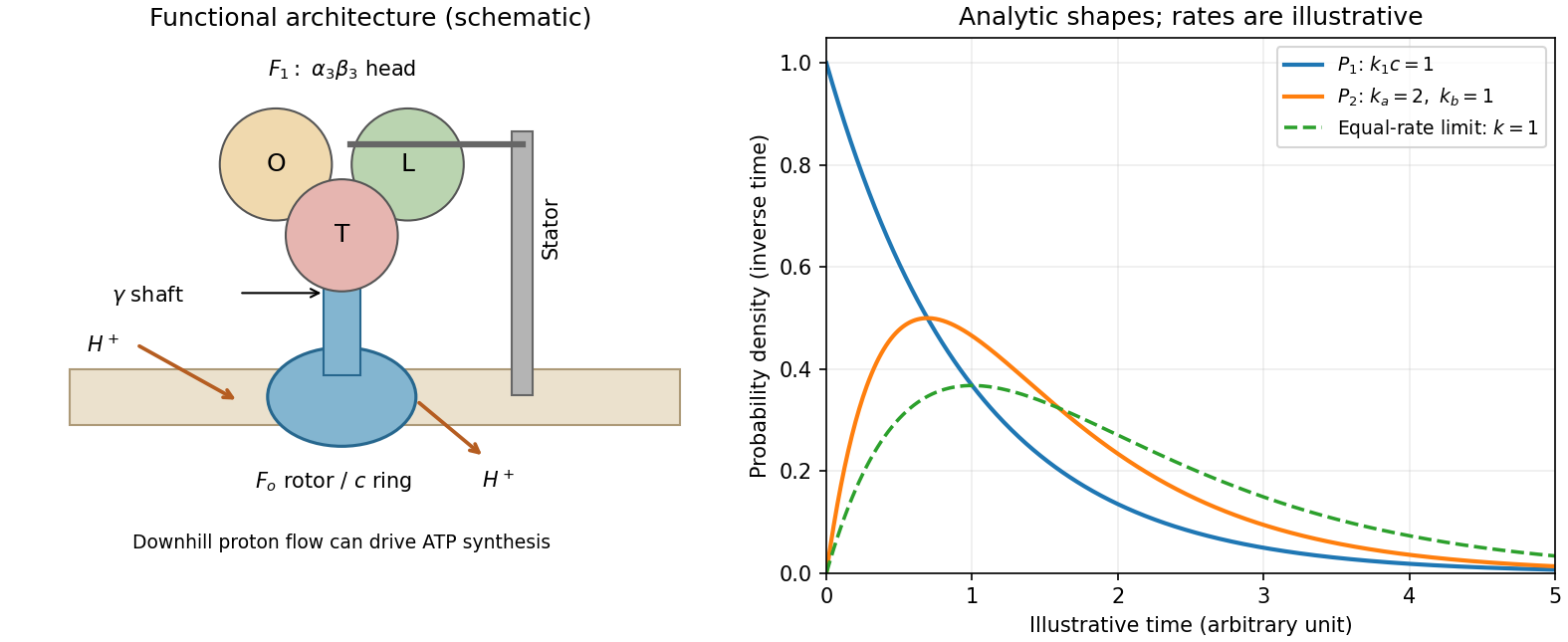
Let $S_1(t)$ be the probability that an ATP-waiting state has not yet bound a substrate molecule. A constant bimolecular binding coefficient $k_1$ at fixed ATP concentration $c$ gives a pseudo-first-order hazard $\lambda =k_{1}c$. Thus ${\dot{S}}_1=-\lambda S_1$, $S_1(0)=1$, and the waiting-time distribution isThe probability density function starts at $k_{1}c$ and decreases exponentially. Increasing $c$ shortens the waiting time in inverse proportion. This supports one rate-limiting ATP-binding event before the associated motion, rather than a concentration-independent chemical delay.

For the second delay, consider sequential independent first-order transitions $A{⟶}^{k_a}B{⟶}^{k_b}C$. Their dwell times have exponential distributions. The total waiting time is their sum, so convolution givesIt is normalized, symmetric under exchange of $k_a,k_b$, and hasUnlike one exponential delay, it vanishes at $t=0$, rises initially as $k_a{k}_{b}t$, reaches a maximum at $t_{\mathrm{mode}}=\log (k_a/k_b)/(k_a-k_b)$ and eventually decays at the slower rate. For equal rates the continuous limit is $P_2(t)=k^{2}t{e}^{-kt}$, an Erlang distribution with mode $1/k$. If one rate is much faster than the other, the observed long-time behavior approaches one exponential. The sketch in the preceding section displays these shapes using arbitrary specified rates.

The simplest catalytic cycle compatible with the fits therefore contains an ATP-dependent binding delay and at least two resolvable ATP-concentration-independent kinetic events. Hydrolysis, product release and conformational changes are possible microscopic assignments, but the two-rate fit alone does not uniquely identify them or the order of $k_a$ and $k_b$. If each complete $120^{\circ }$ cycle contains these three waits and step durations are negligible, its mean duration is $(k_{1}c{)}^{-1}+k_a^{-1}+k_b^{-1}$ and the mean revolution rate is the inverse of three times this duration. Multiple catalytic sites can cooperate during that cycle.

TODO: the source PDF's stepping plot is absent. Its individual substep angles, numerical timings and the mapping of plotted dwell labels onto the larger or smaller angular movement cannot be read. The surviving text establishes only the $120^{\circ }$ total step and the existence of a larger and a smaller substep. No numerical rate, missing angle or plotted label is inferred from a different experiment. The distribution derivations and the concentration-dependence inference above are independent of that illustration.

ATP synthase couples downhill proton motion across a cell membrane to synthesis of ATP from ADP and inorganic phosphate. Its membrane-embedded $F_o$ sector contains an $a$ subunit with offset proton-access half-channels and a rotating $c$-subunit ring. Reversible protonation of sites on the ring permits rotation relative to the stationary $a$ subunit. The central rotor transmits this motion through the $\gamma$ shaft to the soluble $F_1$ head. A peripheral stator holds the head relative to the membrane sector. The common bacterial schematic has an ${\alpha }_3{\beta }_3$ head, catalytic sites mainly on the three $\beta$ subunits, and a central $\gamma /ϵ$ rotor; accessory stator components depend on the organism.

The binding-change mechanism cycles the catalytic sites between open, loose-binding and tight-binding conformations. Rotor orientation changes their affinities for ADP, phosphate and ATP; the sites operate out of phase. Tight binding favors formation of bound ATP, and mechanical rotation changes the conformation to permit product release. In the ideal tightly coupled cycle, one revolution gives three catalytic turnovers:The proton count is not universally fixed: an ideal ring with $n_c$ proton-carrying subunits gives $n_c$ protons per revolution and $n_c/3$ protons per synthesized ATP, before additional transport costs.

For a proton moving from side 1 to side 2, its molar electrochemical potential change isThe chemical gradient and membrane electric potential difference together supply the proton-motive force. Synthesis requires the proton free-energy release to meet the positive Gibbs free energy of ATP synthesis. The coupling is reversible: isolated $F_1$ supplied with ATP can hydrolyse it and rotate its shaft, while the intact enzyme can use hydrolysis-driven rotation to pump protons against their gradient. The sketch is structural and schematic; it does not reconstruct the absent stepping trace.

Protein primary structure is the ordered amino acid sequence of a polypeptide, linked by covalent peptide bonds. The approximately planar peptide bond restricts local geometry, while backbone torsion angles give conformational freedom subject to steric exclusion. Protein secondary structure comprises local backbone arrangements, especially the alpha helix, with backbone hydrogen bonds between residues $i$ and $i+4$, and the beta sheet, whose strands are joined by backbone hydrogen bonds. Turns and loops connect these elements. Protein tertiary structure is the full three-dimensional organization of a single chain, often including several protein domains. Protein quaternary structure is the arrangement of multiple chains in a protein complex.

Protein folding is governed by the Gibbs free energy of the chain together with its solvent, not by the chain's energy alone. Folding reduces the chain's conformational entropy, but can gain solvent entropy through the hydrophobic effect, burying nonpolar side chains away from water. Favorable hydrogen bonds, Van der Waals forces, electrostatic interactions and sometimes covalent disulfide bonds stabilize particular structures. Steric repulsion prevents atomic overlap. At fixed temperature and pressure, the native ensemble is favored when its total $\Delta G=\Delta H-T\Delta S$ is lower than competing ensembles. The balance depends on the solvent, pH, salt and ligands. Molecular chaperones help avoid aggregation or kinetic traps; a stable fold is not a perfectly rigid conformation, and some proteins have disordered regions.

For a soluble globular protein, a typical pattern is a nonpolar core and a polar, hydrated surface. A transmembrane protein instead presents nonpolar side chains to the hydrocarbon interior of the lipid bilayer. Membrane-spanning alpha helices satisfy their polar backbone groups through internal hydrogen bonds; a roughly membrane-thickness helix commonly contains about twenty residues, depending on tilt and bilayer thickness. Multiple helices can enclose polar channels or binding sites. Membrane-spanning beta barrels likewise expose mainly nonpolar groups outward towards lipid while arranging backbone hydrogen bonds between strands and often lining an aqueous pore with polar groups. Exposed loops and domains contacting water can resemble soluble proteins. Not every membrane-associated protein spans the membrane: peripheral attachment and lipid anchoring are distinct possibilities.

The organizing distinction is the environment of each surface: water favors accessible polar groups, while the membrane core favors outward-facing nonpolar groups. Buried polar groups can still be essential to a transport pathway or catalytic site.

The Gamma function identity $\Gamma (1/2)=\sqrt{\pi }$ gives the Bromwich integral of an inverse square root directly:Equivalently, put $x=u^2$ in the real integral. It becomes $2{\int }_0^{\infty }{e}^{-u^2}du=\sqrt{\pi }$ by the Gaussian integral.

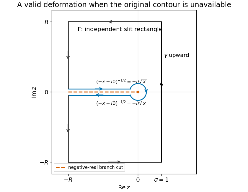
TODO: the original closed-contour drawing is absent from the source. The following independent Bromwich contour deformation establishes the required discontinuity relation without asserting the missing drawing's exact geometry. Orient the vertical line upward, as required by the positive imaginary answer in the next part, and use the principal square root, $-\pi <\arg z<\pi$.

Close a truncated vertical line to the left with a rectangle, slit it along the negative real axis, and exclude a small circle about zero. The integrand is holomorphic inside that slit domain, so the boundary contour integral is zero. Horizontal boundary integrals are $O(R^{-1/2})$: integrating $e^x$ along $-R\le x\le 1$ gives a bounded factor while $|z{|}^{-1/2}\le R^{-1/2}$. The left boundary contributes $O(e^{-R}{R}^{1/2})$, and the small circle contributes $O(\sqrt{\epsilon })$. All vanish in the indicated limits.

At $z=-x$ with $x>0$, the upper and lower bank values are respectively $-i{e}^{-x}/\sqrt{x}$ and $+i{e}^{-x}/\sqrt{x}$. The boundary follows the upper bank toward zero and the lower bank away from zero. Their combined contribution is $-2i{\int }_0^{\infty }{e}^{-x}{x}^{-1/2}dx$. HenceThe vertically improper integral converges conditionally; these estimates also justify the contour limit. Reversing the vertical orientation reverses its sign.

The square-root branch points are zero and infinity. At zero the local behavior is $z^{-1/2}$; in the coordinate $u=1/z$ near infinity it is $u^{1/2}$. In either case one circuit reverses the sign and two restore it. Thus the ramification index is $2$: these are two-sheeted algebraic branch points, sometimes described as branch order one when order means ramification index minus one. The decay to zero at infinity does not remove the branching.

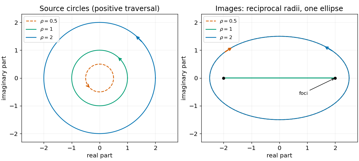
For a radius $\rho >0$, write $z=\rho e^{i\theta }$. ThenFor $\rho \ne 1$ its image is the ellipseIts horizontal semiaxis is $\rho +{\rho }^{-1}$, its vertical semiaxis is $|\rho -{\rho }^{-1}|$, and its foci are $\pm 2$ because the squared semiaxes differ by $4$. Reciprocal radii give the same ellipse, traversed in opposite directions as $\theta$ increases.

For $z=e^{i\theta }$ the image is $w=2\cos \theta$, a real number. Therefore each semicircle maps onto the real interval $[-2,2]$, with endpoints included for closed semicircles. Under positive traversal of the full unit circle, the upper half runs from $2$ to $-2$ and the lower half returns from $-2$ to $2$. Every interior point has two unit-circle preimages. The Joukowski circle-to-ellipse mapping degenerates to a doubled line segment at this radius.

Put $z=1+\zeta$. Expanding the holomorphic function near its critical point givesFor a small ray $\zeta =r{e}^{i\theta }$, the leading image displacement is $r^2{e}^{2i\theta }$. Thus oriented ray angles are doubled modulo $2\pi$ at $z=1$. This is angle multiplication at a holomorphic critical point of multiplicity two; an unoriented angle between full tangent lines must also be interpreted modulo $\pi$. The map is not locally one-to-one there.

The Joukowski map $f(z)=z+z^{-1}$ is holomorphic on $\mathbb{C}\setminus \{0\}$. A holomorphic function is locally conformal where its derivative is nonzero. Here $f^{\prime }(z)=1-z^{-2}$ vanishes at $z=\pm 1$. Thereforewhere the exclusion of zero is because the function is undefined there. Holomorphy alone does not supply conformality at the two critical points.

Parametrize the positively oriented unit circle by $z=e^{i\theta }$. Then $e^{-1/z}=e^{-\cos \theta +i\sin \theta }$ and $dz=i{e}^{i\theta }d\theta$, soEquating the real part and imaginary part with $-2\pi i$ gives

The coefficient of $z^{-1}$ in the Laurent series is $-1$. The residue theorem therefore gives, for the standard positive orientation,The residue theorem applies to an isolated essential singularity as well as to a pole.

The Laurent series isIts principal part contains infinitely many nonzero negative powers, so zero is an essential singularity. The first three displayed terms are not an asymptotic truncation as $z\to 0$; they are the beginning of the convergent Laurent series in powers of $1/z$.

For $|x|\ll s_0$ the quadratic Hamiltonian describes a simple harmonic oscillator withAn exactly circular orbit closes for every nonzero $l$. A nonzero infinitesimal radial oscillation closes at leading order precisely when $\sqrt{3}\sin \theta$ is rational. This condition concerns the cone angle: changing $s_0$ or $l$ cannot change the leading-order ratio. Thus there are no special nonzero $l$ values selecting closure for a fixed cone at this order.

At finite radial amplitude the system is equivalent, after unrolling the cone with planar angle $\chi =\varphi \sin \theta$, to a planar central force with potential proportional to $s$. Its angle advance per radial period changes continuously from $2\pi /\sqrt{3}$ near a circle towards $\pi$ at very large radial energy. Hence the physical advance changes from $2\pi /(\sqrt{3}\sin \theta )$ towards $\pi /\sin \theta$. This nonzero interval contains rational multiples of $2\pi$, so tuning a larger initial $|p_s|$ can produce closed orbits even when the small-amplitude ratio is irrational. Generic amplitudes still produce a precessing orbit; neither energy conservation nor increasing $|p_s|$ guarantees closure.

For fixed nonzero $l=p_{\varphi }$, the radial effective potential is $V_{\mathrm{eff}}(s)=l^2/(2m{s}^2{\sin }^2\theta )+mgs\cos \theta$. Its stationary point isThe equilibrium is therefore stable. A Taylor expansion with $x=s-s_0$ and $p_x=p_s$ givesQualification: the printed “any” $p_{\varphi }$ excludes a regular interior equilibrium when $p_{\varphi }=0$. In that case $V_{\mathrm{eff}}=mgs\cos \theta$ has no stationary point for $s>0$. Its minimum is the nonsmooth apex, where these coordinates and the smooth-cone dynamics fail.

To match the printed order $df/dt=\{H,f\}$, define the Poisson bracket with the sign conventionHamilton's equations imply $\dot{f}={\sum }_i(f_{q_i}{H}_{p_i}-f_{p_i}{H}_{q_i})=\{H,f{\}}_{\mathrm{paper}}$. With the other common Poisson bracket convention the correct statement is instead $\dot{f}=\{f,H{\}}_{\mathrm{standard}}$. For example $H=p^2/(2m)$, $f=q$ gives $\{H,q{\}}_{\mathrm{standard}}=-p/m$, contradicting the printed order unless its sign convention is adopted. Since $H_t=0$ and $\{H,H\}=0$, the Hamiltonian is conserved. Also ${\dot{p}}_{\varphi }=-H_{\varphi }=0$: this canonical momentum is the axial angular momentum.

For a regular Lagrangian, form the canonical momenta $p_i=L_{{\dot{q}}_i}$, invert for ${\dot{q}}_i(\mathbf{q},\mathbf{p},t)$, and take the Legendre transform $H={\sum }_i{p}_i{\dot{q}}_i-L$. On the upper cone let $s>0$ be distance along a generator from the apex and $\varphi$ the azimuth. Then the horizontal radius is $s\sin \theta$ and height is $s\cos \theta$, soConsequently

Let $m$ be the ice mass for which the stated drag coefficients are defined, $K=k_1+k_2$ and $f=2\Omega \sin \ell$. With stationary water, the steady horizontal ice equations areThe linear system givesFor fixed wind speed $V=10\mathrm{m}{\mathrm{s}}^{-1}$, the Cauchy-Schwarz inequality minimizes this component whenThus the wind must blow towards a direction east of south by ${\tan }^{-1}(mf/K)$ in the northern hemisphere, west of south in the southern hemisphere, and due south at the equator. This compensates the Coriolis force; at the optimum $v_x=0$ and the ice moves due south. If the drag coefficients are per unit mass, replace $K/m$ by the corresponding total drag rate. “Blows towards” avoids the opposite convention used when naming winds by their origin.