Annual conversion is reduced by several multiplicative losses. Only roughly $40$–$50\%$ of incident sunlight lies in the photosynthetically useful visible band. Reflection and transmission prevent complete absorption; the photon budget and unavoidable relaxation losses limit conversion of absorbed radiation into chemical energy. Photosynthesis also has to support respiration and maintenance, while seasonal growth, incomplete canopy cover, water and nutrient limitations reduce the annual harvested yield.

An illustrative loss budget, not a universal biological constant, is $0.45\times 0.8\times 0.25\times 0.5\times 0.11\simeq 0.005$. The factors represent useful spectrum, absorption, photochemical conversion, retained net production, and combined annual interception and growing-condition limitations, respectively. Thus $\boxed{{\eta }_{\mathrm{annual}}\sim 0.5\%}$ is plausible for a land-averaged crop yield even though a leaf under favourable illumination can be more efficient. The result depends on crop, climate, harvested fraction and the definition of dry biomass energy. When the input is already annual mean insolation, night-time must not be counted as a second independent loss.

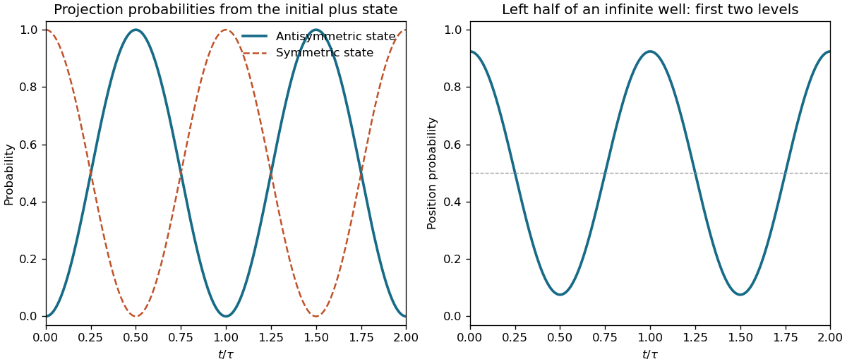
Choose the infinite well as $0<x<a$ with real eigenfunctions ${\psi }_n=\sqrt{2/a}\sin (n\pi x/a)$. This fixes the relative phase convention for the specified initial plus state. Each of the first two states has probability $1/2$ in the left half. Their cross integral isThe evolving superposition therefore givesSince $E_n=n^2{\pi }^2{\hslash }^2/(2m{a}^2)$, the angular frequency and ordinary frequency areThe probability varies between $1/2\pm 4/(3\pi )$ and remains in $[0,1]$. Changing the sign convention of one eigenfunction while keeping the same physical initial state requires changing its superposition coefficient too; otherwise one has prepared the other initial state and reversed the initial spatial bias.

An ideal projective measurement yielding the antisymmetric state prepares that state at $t_1$. Starting from it, the probability of reaching the symmetric state after an additional interval $s$ is again ${\sin }^2((E_2-E_1)s/(2\hslash ))$. At the full recurrence interval found above,The full-period propagator is proportional to the identity on the two-dimensional subspace, so it returns the antisymmetric state to itself, not to its orthogonal partner. The result assumes the stated time-independent evolution continues after the measurement.

Projection onto the antisymmetric quantum superposition gives amplitude $\frac{1}{2}(e^{-i{E}_{1}t/\hslash }-e^{-i{E}_{2}t/\hslash })$. Its squared modulus isIt vanishes initially, reaches one at a half-recurrence time, and returns to zero after $\tau$. This interference depends on a relative phase even though each energy-eigenstate population and the mean energy remain constant.

Each energy eigenstate acquires its own phase under the time-independent Hamiltonian operator:Orthonormality removes all off-diagonal terms from the expected value of the energy, givingReturn up to an overall phase requires the relative phase to return to one. For $E_1\ne E_2$, the shortest positive recurrence time isIf the two energies coincide, the whole superposition is stationary up to a common phase for every time; there is then no smallest strictly positive recurrence time. A half-period changes the relative sign and produces the orthogonal antisymmetric state rather than the original symmetric state.

The wave function is a probability amplitude: by the Born rule, $|\psi (x){|}^{2}dx$ is the probability of a position measurement in an interval of width $dx$. For a normalized bound state $\int |\psi {|}^{2}dx=1$, the expected values areThe integrals run over the allowed domain. If the given state is not normalized, divide both by $\int |\psi {|}^{2}dx$. Its variance is $⟨x^2⟩-⟨x{⟩}^2$; neither $\psi$ itself nor its overall phase is a directly measured position probability.

The one-dimensional time-independent Schrödinger equation isThe differential term is the kinetic energy operator acting on the wave function, $V(x)$ supplies the multiplicative potential energy, and their sum is the Hamiltonian operator. The eigenvalue $E$ is the stationary state's total energy. This form assumes a nonrelativistic particle, a time-independent scalar potential, and no additional internal degrees of freedom in the stated model.

For Coulomb binding, the virial theorem gives a typical kinetic energy of the order of the binding energy. Taking $p_{\mathrm{typ}}\simeq \sqrt{2m_e|E_1|}$ and using the Heisenberg uncertainty relation estimate $r_{\mathrm{typ}}\sim \hslash /p_{\mathrm{typ}}$ givesThe Bohr model gives $r_1=a_0/Z=a_0/2=2.65\times 10^{-11}\mathrm{m}$ for a heavy helium nucleus, agreeing with the characteristic scale. Equivalently, minimizing the localization estimate $E(r)\sim {\hslash }^2/(2m_e{r}^2)-Z{e}^2/(4\pi {ϵ}_{0}r)$ gives that same scale.

This is an order-of-magnitude radius estimate, not an exact deduction of the cloud's expected value from the inequality alone. Numerical coefficients depend on which spread is used; $\Delta x\Delta p\ge \hslash /2$ does not assert $⟨r⟩=\hslash /p$. For the exact hydrogenic $1s$ state, $⟨r⟩=3a_0/(2Z)=3.97\times 10^{-11}\mathrm{m}$ at $Z=2$, one and a half times the Bohr orbital radius. An electron cloud has a radial distribution, whereas the Bohr model assigns a definite radius.

At room temperature, $k_{B}T$ is of order $0.026\mathrm{eV}$, far smaller than the electronic excitation gaps of the inferred hydrogenic ion. Ground-state absorption is therefore the natural interpretation. Assign the three lines to $1\to 2$, $1\to 3$, and $1\to 4$. Dividing each reciprocal wavelength by its corresponding factor $1-1/n^2$ givesThe small scatter is consistent with the rounded wavelength data. Since $R_{\infty }\simeq 1.0974\times 10^7{\mathrm{m}}^{-1}$ and $\mu \simeq m_e$,The ion is thus hydrogen-like lithium, ${\mathrm{Li}}^{2+}$. If “effective Rydberg constant” denotes only the reduced-mass constant rather than the charge-inclusive spectral coefficient, its value is $R_M\simeq R_{\mathrm{eff}}/9\simeq 1.097\times 10^7{\mathrm{m}}^{-1}$. The two conventions are explicitly distinguished; the rounded lines do not determine a precise isotope mass.

The emitted photon carries the decrease in atomic energy, so $hc/\lambda =E_n-E_m$ for $n>m$. Using the preceding energy levels givesThe lower state's energy is more negative, making the right-hand side positive. This is the hydrogenic Rydberg formula, with the finite-nuclear-mass factor included in $R_M$.

Let $r$ be the electron-nucleus separation and use the reduced mass $\mu =m_{e}M/(m_e+M)$. Coulomb attraction supplies the relative centripetal force, and Bohr quantization fixes the relative angular momentum:Eliminating $v$ givesThe total energy is $E=\mu v^2/2-Z{e}^2/(4\pi {ϵ}_{0}r)=-Z{e}^2/(8\pi {ϵ}_{0}r)$, henceHere $a_0$ is the ordinary Bohr radius and $R_{\infty }$ the infinite-nuclear-mass Rydberg constant. The electron's radius about the centre of mass is $M{r}_n/(M+m_e)$; for a heavy nucleus this distinction and the reduced-mass correction are small, but the supplied nuclear mass permits them to be stated precisely.

A classical orbiting electron accelerates and therefore radiates according to the Larmor formula. Its mechanical energy becomes more negative, its radius decreases, and the orbit spirals inward rather than remaining a stable atom. The Bohr model replaces this prediction with postulated nonradiating stationary states and quantized orbital angular momentum, together with photon emission or absorption only between states, $h\nu =|E_n-E_m|$.

For a heavy nucleus, $m_{e}vr=n\hslash$. Since the de Broglie wavelength is $h/(m_{e}v)$, this impliesThe electronic wave fits an integer number of wavelengths around the orbit. This is a standing-wave consistency interpretation of the quantization rule, not a classical mechanism that prevents an accelerating charge from radiating. For finite nuclear mass, the two-body relative coordinate uses reduced mass $\mu =m_{e}M/(m_e+M)$; the next derivation retains that correction. In the limit $M\gg m_e$, it reduces to the fixed-nucleus electron description above.

In the Franck-Hertz experiment, electrons emitted from a heated cathode are accelerated through a dilute atomic vapour toward a collector. A small retarding potential before the collector rejects electrons that have lost too much kinetic energy. Below the first excitation threshold, mainly elastic collisions occur and the collector current rises as the accelerating voltage increases. At threshold an inelastic collision can transfer a definite excitation energy to an atom, causing a current drop because the slowed electron cannot overcome the retarding potential.

Raising the voltage further permits acceleration again, and repeated losses produce successive current minima. For mercury their spacing is about $4.9\mathrm{V}$, corresponding to an atomic excitation of about $4.9\mathrm{eV}$ and an associated ultraviolet photon near $254\mathrm{nm}$. Contact potentials shift the absolute voltages, so the spacing is more informative than the first minimum's position alone. Discrete energy losses support discrete atomic energy levels; a continuously variable excitation energy would not produce the same recurring fixed loss scale. The experiment establishes quantized excitations without requiring the classical electron orbit of the Bohr model to be literally correct.

For nonrelativistic neutrons, $\lambda \propto E_K^{-1/2}$, so first-order uncertainty propagation gives $|\Delta \lambda |/\lambda =\frac{1}{2}|\Delta E_K|/E_K=0.05$. ThusAt fixed $d$, differentiating the stipulated first-order relation $d\sin \theta =\lambda$ gives $\Delta \theta =\tan \theta \Delta \lambda /\lambda$. ConsequentlyFor photons, $\lambda \propto E^{-1}$, so the same fractional energy uncertainty gives $\Delta {\lambda }_{\gamma }/{\lambda }_{\gamma }=0.10$. Their $18.8\mathrm{keV}$ wavelength almost equals the low-energy neutron wavelength, so the conditional central angle is $0.116973\mathrm{rad}$ andabout twice the neutron angular spread. This difference comes from the different energy-momentum relations, not from substantially different central wavelengths. The small-angle approximation is adequate at $0.117\mathrm{rad}$: replacing $\sin \theta$ by $\theta$ changes it by about ${\theta }^2/6=0.23\%$, and replacing $\tan \theta$ by $\theta$ changes the sensitivity by about $0.46\%$. The numerical angular results retain the preceding geometry qualification; a different physical scattering geometry would require its own angle convention.

For a transverse periodic row of scatterers of spacing $d$, normal incidence makes their incident phases equal. Scattering at angle $\theta$ from that normal creates an outgoing path difference $d\sin \theta$ between neighbours. Constructive interference requires a phase difference $2\pi n$, givingUsing this printed relation as the intended transverse diffraction grating model, the nonrelativistic neutron wavelength at $0.188\mathrm{eV}$ is $\lambda =6.5964\times 10^{-11}\mathrm{m}$. Hence the first-order data giveGeometry qualification: this is not a derivation from reflection at crystal planes parallel to the surface, as the source prose says. The ordinary Bragg's law for planes of normal separation $d$ is $2d\sin {\theta }_B=n\lambda$, where ${\theta }_B$ is the incident glancing angle to those planes. At normal incidence on parallel planes, ${\theta }_B=\pi /2$ and specular reflected rays leave along the normal, so their angle from the normal is zero; they cannot obey the printed positive-order relation $d\sin 0=n\lambda$ for $\lambda >0$. This is a concrete counterexample to identifying the two geometries. The numerical spacing above is therefore conditional on the printed grating-like relation, rather than a forced assertion that the stated Bragg geometry proves it.

For a photon, $p_{\gamma }=E/c$ and ${\lambda }_{\gamma }=hc/E$. The neutron is nonrelativistic here because $18.8\mathrm{keV}\ll m_n{c}^2$, so $p_n=\sqrt{2m_{n}E}$ and ${\lambda }_n=h/p_n$. Using the supplied common energy givesEqual kinetic energies do not imply equal momenta: the massive particle obeys $E=p^2/(2m_n)$, while the massless photon obeys $E=pc$. The neutron momentum is about $316$ times larger, so its de Broglie wavelength is about $316$ times smaller.

To give the neutron the photon wavelength, set its momentum to $E/c$, not its kinetic energy to $E$ again. ThenIts kinetic energy would then be about $0.188\mathrm{eV}$, connecting this comparison with the next calculation.

Black-body radiation and the photoelectric effect exposed failures of classical continuous-wave energy exchange. Classical equipartition predicted an unbounded short-wavelength thermal spectrum, the ultraviolet catastrophe. Quantized oscillator energies $E_n=nh\nu$ give the mean excitation energy $h\nu /(e^{h\nu /(k_{B}T)}-1)$ and suppress high-frequency modes, producing Planck's law. In the modern description, thermal radiation consists of photons with energy $h\nu$ and Bose occupation numbers.

For the photoelectric effect, increasing intensity below a threshold frequency does not eject electrons, whereas the maximum electron kinetic energy grows with frequency above threshold. Absorption of one photon transfers $h\nu$ to one electron, giving $\boxed{K_{\max }=h\nu -W}$ and threshold ${\nu }_0=W/h$, where $W$ is the work function. Intensity primarily changes the photon arrival rate and hence the photocurrent in the ordinary single-photon regime. Thus changing energy per quantum and changing the number of quanta have distinct consequences. Historically the thermal derivation first quantized matter's energy exchange; it should not be described as an already complete derivation of modern photon theory.

For a spherical mass distribution with constant circular speed $v_c$,For $v_c=220\mathrm{km}{\mathrm{s}}^{-1}$, this is about $0.0140(r/8\mathrm{kpc}{)}^{-2}{M}_{\odot }\mathrm{p}{\mathrm{c}}^{-3}$. It is the spherical model's total density; it is singular if extrapolated to the very centre and is intended only over the flat-rotation region.

For a sharp outer truncation at $r_{\ast }$, the exterior mass is fixed at $M_{\ast }=v_c^2{r}_{\ast }/G$. Integrating the gravitational work from $r$ to the boundary and then to infinity givesThusThe exterior contribution cannot be dropped: at $r=r_{\ast }$ it correctly gives the point-mass escape speed $\sqrt{2}{v}_c$.

If the fastest measured radial speed is assumed to approximate both the total speed and the local escape speed of a bound star, then at $r=8\mathrm{kpc}$,Without those extra assumptions, the measurement gives only a bound: a bound star's total speed is at least its radial component, and the sample maximum need not reach escape, so $r_{\ast }\gtrsim 19.9\mathrm{kpc}$ within this model. An unbound interloper would invalidate even that bound. This is not a determination of the real Milky Way halo edge.

Use a Tully-Fisher relation $L\propto v_{\max }^4$. A simple justification assumes comparable mean surface brightness, so $L\propto R^2$, and comparable total mass-to-light ratio, so $M\propto L$. The virial scaling $v^2\sim GM/R$ then gives $v^4\propto M^2/R^2\propto L$. Calibrating to the previous galaxy yieldsThis is a rough luminosity estimate: the empirical slope depends on passband and population, and the assumed constant surface brightness and mass-to-light ratio are approximations rather than exact properties of every spiral galaxy.

Use the low-redshift Hubble law, neglecting peculiar velocity and cosmological distance corrections:The angular radius is $15$ arcseconds, half the stated major-axis diameter. A spherical dynamical estimate givesIt estimates mass inside the observed disk radius, not the entire unobserved halo. Disk geometry changes the exact coefficient.

Using the same approximate distance for the distance modulus,For an illustrative stellar mass-to-light ratio of $1$--$5$ in solar $V$-band units, $M_{\ast }\sim 1.5\times 10^{10}$--$7.4\times 10^{10}{M}_{\odot }$, below the dynamical estimate. This suggests substantial nonluminous matter under the adopted assumptions. Gas, stellar-population uncertainty, inclination, extinction and geometry also affect the comparison; luminosity alone cannot uniquely fix a stellar mass. The single-distance approximation at $z\simeq 0.05$ is the intended introductory estimate.