Put $A=b_1{E}_0/b_0$. The proposed solution can be writtenIt gives $C(0)-C_0=A$. Differentiation and substitution give, respectively,so it satisfies both the differential equation and the initial condition. At $t=200$ years,with $E(2000)=0.02e^6\simeq 8.069\mathrm{GtC}\mathrm{y}{\mathrm{r}}^{-1}$. The earlier emissions grow on the $g^{-1}=33.3$ year timescale, much faster than the model's 200-year removal time.

The term $b_{1}E$ is the effective atmospheric addition from ongoing emissions. Its coefficient $0.25ppmv/GtC$ is about half the full-retention estimate $0.47ppmv/GtC$, so the model implicitly removes or partitions some emitted carbon promptly. The term $-b_0(C-C_0)$ represents slower net uptake of the excess by other reservoirs; its relaxation time is $b_0^{-1}=200$ years. Both terms have units of ppmv per year.

Thousands of years at constant $E_0$ erase the initial transient, givingThe reference $C_0$ is the zero-anthropogenic-emission equilibrium, not the equilibrium when the stated small persistent emissions are present.

Complete oxidation of $10^{12}\mathrm{kg}$ of carbon adds $n_C=10^{12}/(12\times 10^{-3})=8.33\times 10^{13}\mathrm{mol}$ of carbon dioxide. With atmospheric mass about $5.1\times 10^{18}\mathrm{kg}$ and mean air molar mass $28.97\times 10^{-3}\mathrm{kg}\mathrm{mo}{\mathrm{l}}^{-1}$, there are about $1.76\times 10^{20}\mathrm{mol}$ of air. The dry-air mole fraction, approximately the volume fraction, changes byIt is the carbon inventory that counts: oxidation adds oxygen to each molecule but does not change the number of carbon-containing molecules. Using $5.15\times 10^{18}\mathrm{kg}$ instead changes the estimate by only about one percent. The atmospheric constants are standard Earth estimates, not additional data read from a missing plot.^[ref]

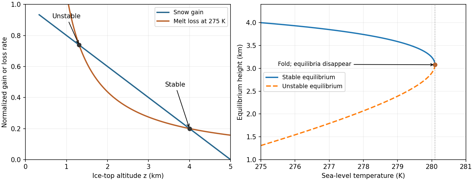
At $z=4\mathrm{km}$, the snow gain is $1-0.2(4)=0.2$ and the model's top Celsius temperature is $275-273.15-6(4)=-22.15^{\circ }\mathrm{C}$. Equilibrium givesin the normalized rate convention. Using $273\mathrm{K}$ for the Celsius zero instead would give $4.4^{\circ }\mathrm{C}$. The local slope is $-0.2+4.43(6)/(22.15{)}^2\simeq -0.1458\mathrm{k}{\mathrm{m}}^{-1}<0$, as required. Initially $z_{-}=1.3083\mathrm{km}$ and $z_{\mathrm{slope}}\simeq 2.230\mathrm{km}$, while $z_{+}=4\mathrm{km}$.

As $T_s$ slowly rises, melt loss increases at fixed $z$, the stable high branch moves downward and the unstable branch upward. They merge atBeyond the fold the model has no steady cold ice cap: its net balance is negative throughout the physical interval and ice shrinks until the assumed law ceases to apply. Quasistatic tracking presumes adjustment is fast compared with the imposed warming, an assumption that deteriorates near the fold as the restoring slope tends to zero. This singular idealized law is not a quantitative real-world melting forecast.

Write $s=T_s-273.15\mathrm{K}$ as the numerical sea-level Celsius temperature in degrees Celsius, and use the same degree increments for $\Gamma z$. The model's top temperature is $T_C=s-\Gamma z$. For positive $\alpha$ its intended cold-ice branch has $T_C<0$, so the positive melt-loss magnitude and snow gain areThe model is singular at $z=s/\Gamma$ and is not a physical melting law across that boundary. On the relevant interval $s/\Gamma <z<1/\beta$, $L$ decreases hyperbolically and $A$ decreases linearly. Assume a fixed area and positive ice density, so increasing mass increases $z$: stability has the same sign as $F^{\prime }(z)$.

The equilibrium equation iswith rootsTwo distinct physical equilibria, one stable, exist providedThis combines a positive allowed interval with a strictly positive discriminant. At the larger root $F^{\prime }<0$ and small perturbations restore the ice cap; the smaller root has $F^{\prime }>0$ and is unstable. Sincea restoring local response requiresThis is the lower height bound from the stability derivative; the stable equilibrium itself is $z_{+}$. The minimum initial height for persistence, a different notion of threshold, is the unstable separator $z_{-}$: initial heights above it approach $z_{+}$, while lower heights lose ice and leave the model's cold branch. At equality in the discriminant condition the two equilibria merge, giving a marginal fold rather than a strictly stable ice cap.

Hydrostatic equilibrium balances the vertical pressure gradient against weight, $dP/dz=-\rho g$. For a dry ideal gas parcel displaced slowly enough to maintain pressure balance but rapidly enough to exchange negligible heat, the first law givesCombining the two equations yields the dry adiabatic lapse rateusing $c_p\simeq 1004\mathrm{J}\mathrm{k}{\mathrm{g}}^{-1}{\mathrm{K}}^{-1}$. Here temperature in the thermodynamic differential is absolute, $g$ and $c_p$ are treated as constant, composition is fixed, and condensation is excluded. Hydrostatic balance alone does not force the atmosphere to be adiabatic; the parcel assumption supplies the extra relation.

Water condensation releases latent heat, reducing the cooling of a rising saturated parcel and giving a smaller moist adiabatic lapse rate. Radiation, mixing, large-scale motion and incomplete convective adjustment also shape the environmental lapse rate. Thus an observed $6$--$7\mathrm{K}\mathrm{k}{\mathrm{m}}^{-1}$ need not equal the dry parcel value and is broadly consistent with a moist, radiatively influenced atmosphere.

Use the optical-depth weighting stipulated in the paper. A jump in the Planck function at ${\tau }_1$ gives $dB/d\tau =(B_1-B_0)\delta (\tau -{\tau }_1)$, soThe upper isothermal layer emits $\pi B_0(1-e^{-{\tau }_1})$ and transmits the lower region's blackbody spectral irradiance with factor $e^{-{\tau }_1}$. The lower layer and black surface have the same $B_1$, so their combined radiation entering the upper layer is $\pi B_1$, independent of how its emission is divided between the lower gas and surface.

More generally, integration by parts rewrites the supplied expression asThe terms are attenuated surface emission and the atmosphere's own emission. In the original boundary-plus-gradient form, $\pi B_0$ is the isothermal reference flux and the integral corrects for temperature variation below the top. Optical depths of order unity contribute most strongly. These formulas follow the paper's specified exponential weighting; a full angular radiative transfer calculation uses ray-angle-dependent optical paths rather than identifying every ray with a vertical path.

Spectral irradiance $F_{\lambda }$ is radiant power crossing unit area per unit wavelength, integrated over the relevant hemisphere with the projected-area factor: $F_{\lambda }=\int I_{\lambda }\cos \theta d\Omega$. Its units are $\mathrm{W}{\mathrm{m}}^{-2}$ per unit wavelength; spectral radiance $I_{\lambda }$ additionally refers to unit solid angle. For an isotropic outgoing hemisphere with Planck function $B_{\lambda }$, the integral is $F_{\lambda }=\pi B_{\lambda }$.

The vertical optical depth above height $z$ is the dimensionless extinction integralHere $z$ increases upward, $n_a$ is absorber number density, ${\sigma }_{\lambda }$ its absorption cross section, ${\rho }_a$ its mass density, and ${\kappa }_{\lambda }$ the absorption coefficient per unit absorber mass. Equivalently, using bulk air density $\rho$ and absorber mass fraction $q_a$, $d{\tau }_{\lambda }/dz=-{\kappa }_{\lambda }{q}_a\rho$. The coefficient may depend on temperature, pressure and wavelength. For purely absorbing gas, transmission along a ray is $e^{-{\tau }_{\mathrm{ray}}}$; scattering, if present, contributes to extinction and requires its own source term.

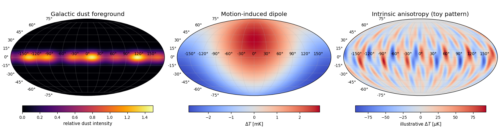
After subtracting the mean, the motion-induced dipole and galactic foregrounds, intrinsic Cosmic microwave background anisotropy appears as angular hot and cold patches, typically at the $10^{-5}$ fractional scale. These spatial temperature fluctuations encode early density and velocity structure. The displayed patch pattern is illustrative, with no claim to reproduce an observed sky map.

Observer motion produces the cosmic microwave background dipole: to first order in $\beta =v/c$,The direction of motion is hotter and the opposite direction cooler. Its full-sky pattern has one broad positive hemisphere and one broad negative hemisphere; it is not concentrated in the galactic plane.

Thermal interstellar dust produces a bright galactic foreground concentrated toward the Milky Way plane, with additional cloud structure. Its emission spectrum differs from the approximately $2.73\mathrm{K}$ blackbody spectrum of the cosmic microwave background, so comparisons across frequencies help separate it. In the sketch below this is the bright equatorial band.

Convert both inputs to energy density. The matter contribution, including rest energy, is $u_{M,0}={\rho }_{M,0}{c}^2=2.25\times 10^{-10}\mathrm{J}{\mathrm{m}}^{-3}$. The given photon value is $u_{\gamma ,0}=5\times 10^5(1.602\times 10^{-19})=8.01\times 10^{-14}\mathrm{J}{\mathrm{m}}^{-3}$. HenceMatter energy density scales as $(1+z{)}^3$, whereas the cosmic microwave background scales as $(1+z{)}^4$. The photon-only matter-radiation equality condition is thereforeThis uses the supplied CMB photon density. Additional relativistic species change equality for total radiation.

Adiabatic expansion preserves the blackbody form while each photon's energy redshifts as $a^{-1}$. Thus the cosmic microwave background temperature obeys $T(z)=T_0(1+z)$, giving

The stated one-sided temperature contrast is $\beta =0.00105$, so the Doppler dipole givesThe motion is toward the hotter region. The contrast already gives one side relative to the mean; the hot-to-cold difference would be twice as large.

Measure the absolute spectral radiance over a range of frequencies and fit the Planck spectrumFor example, the COBE FIRAS blackbody spectrum experiment used a differential Michelson interferometer to compare the sky with an internal blackbody; an external calibrated blackbody could cover the sky entrance. Cold bolometers measured the difference spectrum, and foreground separation distinguished Milky Way emission from the nearly isotropic background. The fitted background temperature is approximately $\boxed{T_0=2.73\mathrm{K}}$.^[ref] The result relies on an absolute spectral comparison, rather than merely measuring a map's hot-to-cold contrast.

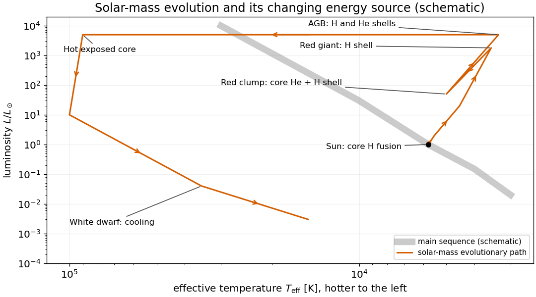
A Hertzsprung-Russell diagram plots stellar luminosity upward and effective temperature increasing toward the left. The main sequence runs from hot luminous stars at upper left to cool faint stars at lower right, with the Sun near $T_{\mathrm{eff}}\simeq 5800\mathrm{K}$, $L=L_{\odot }$.

In the evolution of a solar-mass star, core hydrogen fusion initially supplies the luminosity. As core hydrogen is exhausted, hydrogen-shell fusion around a contracting helium core carries the star through the subgiant and red giant phases toward higher luminosity and lower surface temperature. Helium ignition is followed by core helium fusion with a hydrogen-burning shell, placing a solar-mass star in the red clump. The later Asymptotic giant branch has hydrogen- and helium-burning shells around a carbon-oxygen core. Envelope ejection exposes a hot central star of a planetary nebula; residual shell burning ends and the resulting white dwarf radiates stored thermal energy as it cools.

Use the supplied atomic masses consistently. Their mass defect per four hydrogen atoms is $4(1.0078)-4.0026=0.0286$ atomic mass units. The conversion efficiency isThe atomic-mass bookkeeping includes the associated positron-annihilation energy; an exact photon-heating budget also subtracts energy carried away by neutrinos. With the stated ten-percent fuel fraction and constant present solar luminosity, the main sequence lifetime estimate isThe much longer timescale explains why stellar nuclear fusion can power the Sun throughout its long main-sequence history.

Build the star by adding spherical shells. With $m(r)$ the enclosed mass, its gravitational binding energy isFor a nondegenerate extended star, $r(m)<R_{\odot }$ on the interior, soThis is a gravitational binding-energy lower bound for a spherical star. The Kelvin-Helmholtz cooling time is of orderThe displayed energy bound gives $|\Omega |/L_{\odot }>1.6\times 10^7$ years; it supplies a lower bound on that reservoir-to-luminosity ratio. A stellar structure model sets its coefficient. For an ideal monatomic, gas-supported star the virial theorem puts about half the released gravitational energy into heat, leaving half available for radiation; a uniform-density model would give about $9\times 10^6$ years. These contraction estimates are all of order $10^7$ years, much shorter than the nuclear lifetime.