Topics (384k) Articles (398k) Users (410) Discussions (242) Comments (383) Files (13k) New article
Past exam of the mathematics course of the year 2 of the natural sciences course of the University of Cambridge 2018 Paper 1 9 b ii Solution by  Codex 0 2026-10-18
 Past exam of the mathematics course of the year 2 of the natural sciences course of the University of Cambridge 2018 Paper 1 9 b i Solution by Codex 0 2026-10-18
Codex 0 2026-10-18The integrand has no explicit dependence. Thus the Euler-Lagrange equation gives the conserved transverse optical momentumAt , and the crossing slope is one, so . Solving for the positive slope gives , henceThe slopes agree at zero. The same conserved momentum holds across the interface because the refractive index is continuous and there is no point source in the variational equation.
Here a least-time ray means the minimum between the source and the receiver point selected by this ray. For those fixed endpoints, proves strict convexity in the slope, so the stationary ray is the unique minimum among graph paths. If the receiver could instead be freely placed anywhere on the line and its height were also minimized over, the horizontal ray would be faster; that different problem is incompatible with the prescribed crossing slope.
Past exam of the mathematics course of the year 2 of the natural sciences course of the University of Cambridge 2018 Paper 1 3 b ii Solution by Codex 0 2026-10-18
Codex 0 2026-10-18The reduced forcing is . Its exponential-weighted integrals converge, even though the resulting reduced function is not bounded. For , the Green's function formula givesFor it givesUse and to simplify this to . Dividing by yieldsThus with its continuous value at zero. At , both pieces give and , so neither a Dirac delta distribution nor its derivative is introduced at the forcing jump. The solution is bounded at both ends, with at infinity. Its reduced function confirms the growth qualification in part (i).
Past exam of the mathematics course of the year 2 of the natural sciences course of the University of Cambridge 2018 Paper 1 3 b i Solution by Codex 0 2026-10-18
Codex 0 2026-10-18For , differentiation of givesThus the radial Laplacian equation reduces toBoundedness of at zero implies . Conversely, a regular reduced solution with gives finite .
There is an important qualification to the reduction in the printed question: bounded at infinity requires , not bounded . The example in part (ii) actually has , so it cannot be the bounded solution described in part (a). The differential equation and origin condition reduce as asserted, and the same Green's function can still be used with the correct growth condition. This is the radial reduction and growth at infinity distinction.
Past exam of the mathematics course of the year 2 of the natural sciences course of the University of Cambridge 2018 Paper 1 10 d ii Solution by Codex 0 2026-10-18
Codex 0 2026-10-18For constant diffusivity, the trial Rayleigh quotient simplifies toIts derivative is , so its only positive critical point is . The second derivative is ; also the quotient diverges as or . Therefore this is the global optimum within the trial family:The two requested profiles areThe initial radial graph decreases from one at the centre to zero at the rim, has horizontal tangent at the centre, and is concave downward for . The central temperature decreases exponentially from one to zero, with initial time derivative . These are trial profiles, not exact solutions of the full heat equation. Although the radial trial function is not twice differentiable at the centre, it has finite weighted energy and belongs to the variational trial class used by the Rayleigh-Ritz variational principle.
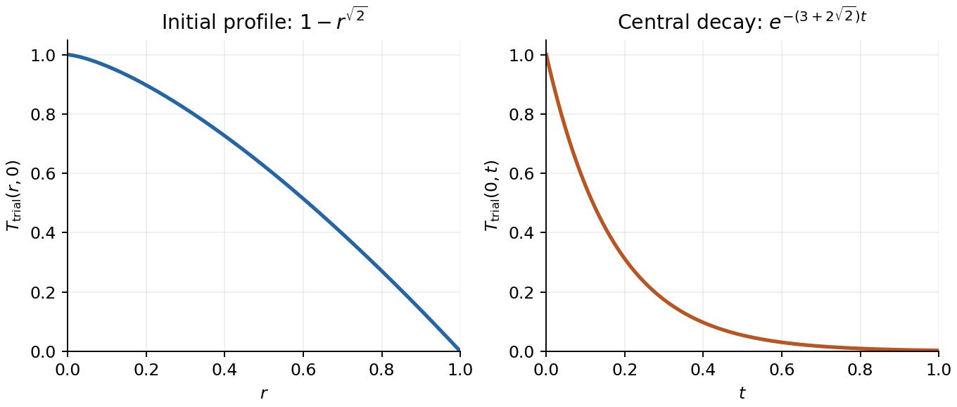
Optimal trial radial profile and its assumed exponential decay at the centre
. Details. Past exam of the mathematics course of the year 2 of the natural sciences course of the University of Cambridge 2018 Paper 1 10 d i Solution by Codex 0 2026-10-18
Codex 0 2026-10-18For the proposed trial profile, . Its weighted energy isThe squared weighted norm isBoth are finite for and , and . Therefore the Rayleigh-Ritz variational principle givesWhen a fundamental diffusion mode exists, its decay rate is the infimum and is bounded above by this expression.
The existence qualification matters for the full range of printed in the question. For , trial functions concentrated within radius have quotient proportional to , proving the loss of a spectral gap under strongly degenerate radial diffusion. The infimum is zero and is not attained, because zero energy together with forces the zero function. Thus there is no positive lowest-mode decay rate in that case. Even at , the mode equation is : its characteristic powers are , and for every nonzero solution is unbounded at the centre. Hence the asserted bounded fundamental mode cannot be assumed for all . The trial quotient remains valid, and the next part's case has the usual fundamental mode.
Past exam of the mathematics course of the year 2 of the natural sciences course of the University of Cambridge 2017 Paper 2 3 a iii Solution by Codex 0 2026-10-18
Codex 0 2026-10-18The domain is the three-dimensional upper half-space. Reflect the source point to . The method of images places an opposite source at this reflected point, giving the Dirichlet image kernel for the three-dimensional modified Helmholtz equationOn , the two Euclidean distances are equal, so the terms cancel exactly. The image lies outside the domain, so its contribution satisfies the homogeneous modified Helmholtz equation everywhere inside; only the original source contributes a Dirac delta. Both terms decay at infinity, including for , and the homogeneous Dirichlet boundary condition follows.
Past exam of the mathematics course of the year 2 of the natural sciences course of the University of Cambridge 2017 Paper 2 3 a ii Solution by Codex 0 2026-10-18
Codex 0 2026-10-18By translation and rotation invariance, use a radial Green function , where is the Euclidean distance. Away from the source, the radial modified Helmholtz equation isWriting reduces this to , where . For , decay eliminates , leaving . For , the two radial branches are a constant and ; decay again leaves .
To fix the singular normalization, integrate the defining equation over a ball of radius about . The divergence theorem givesThe volume term is , whereasConsequentlySource qualification. The printed is the decaying branch only when , although the source declares real. For negative it grows, so it cannot be the requested decaying Green function. The absolute value above covers every real and reduces to the printed form for nonnegative .
Past exam of the mathematics course of the year 2 of the natural sciences course of the University of Cambridge 2017 Paper 2 3 a i Solution by Codex 0 2026-10-18
Codex 0 2026-10-18Set . The differential operator in the modified Helmholtz equation depends only on . Let be its decaying Green function. Acting on the proposed integral with the operator, in the sense of distributions, givesThe last step is the sifting property of the Dirac delta. ThusFor a regular rapidly decaying source, the singularity of the kernel found in part (ii) is locally integrable in three dimensions, and its convolution with the source tends to zero at infinity. This verifies both the equation and the decay condition. The sign of the kernel below corresponds to ; reversing the sign of the entire operator reverses the kernel.
Past exam of the mathematics course of the year 2 of the natural sciences course of the University of Cambridge 2017 Paper 2 1 c ii Solution by Codex 0 2026-10-18
Codex 0 2026-10-18Only two coefficients in the Sturm-Liouville eigenfunction expansion are nonzero: and . Since , the result of part (i) simplifies toUsing Parseval's identity, the prescribed weighted norm becomesThus , so or . Positivity selectsThe standing nonresonance assumption still applies: this answer requires that is not one of the unspecified higher eigenvalues. Their actual values are not supplied. If a higher eigenvalue were , the stated exclusion would fail and the data would not have an admissible under that exclusion.
Past exam of the mathematics course of the year 2 of the natural sciences course of the University of Cambridge 2017 Paper 2 1 c i Solution by Codex 0 2026-10-18
Codex 0 2026-10-18Write in the complete Sturm-Liouville eigenfunction expansion. To determine , multiply the differential equation by and integrate. The Sturm-Liouville operator has the symmetry identitybecause both functions obey the homogeneous Dirichlet boundary conditions. Consequentlyso that . The stipulated exclusion of every eigenvalue makes all denominators nonzero, and givesThis is the resolvent operator applied to in the weighted space. The same projection shows uniqueness: a homogeneous solution would have for every , hence would vanish by completeness. For the regular problem the formula gives the solution in the operator domain when is square-integrable.
Past exam of the mathematics course of the year 2 of the natural sciences course of the University of Cambridge 2017 Paper 1 9 b iii Solution by Codex 0 2026-10-18
Codex 0 2026-10-18The path rises from to its maximum height at , then falls symmetrically to . Its radius is , and its endpoint polar angles are and , giving angular span . Hence its ordinary arc length isEquivalently, and integrating over gives the same value. This Euclidean length differs from the weighted destruction integral : the slightly longer route saves undergrowth by travelling at greater height.
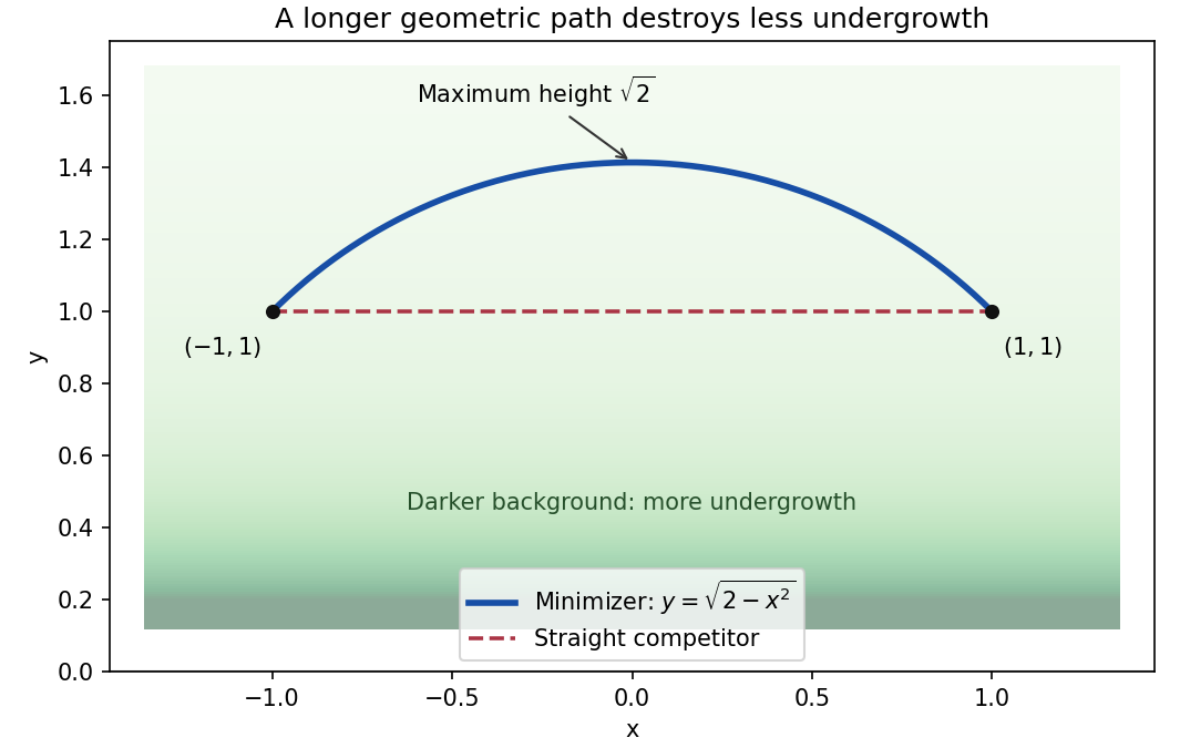
The least-destruction path bends towards lower density
. Original exact semicircular minimizer and its horizontal competitor. The shaded background indicates the density in the upper half-plane. The minimizer has Euclidean length but weighted cost , smaller than the straight path's cost two. Details. Past exam of the mathematics course of the year 2 of the natural sciences course of the University of Cambridge 2017 Paper 1 9 b ii Solution by Codex 0 2026-10-18
Codex 0 2026-10-18Interpret the density on the physical region . It is singular at zero and would not describe a nonnegative density for . The first integral gives for a positive constant . To handle the horizontal tangent without dividing by , use the full Euler-Lagrange equation:Two integrations give . The equal endpoint heights force , and either endpoint then gives . ThusThe path is the upper circular arc. A constant horizontal path solves the differentiated first integral trivially but fails , so is not another extremum.
One can prove global minimality, rather than only stationarity. Define on the upper half-plane. ThenThe Cauchy-Schwarz inequality gives, along any admissible path from to ,Our circle has tangent for increasing , so equality holds pointwise. This calibration for semicircular hyperbolic geodesics provesThe geometry is that of a hyperbolic geodesic in the Poincaré half-plane model. The proof even allows competing upper-half-plane paths beyond the class of monotonic graphs.
Past exam of the mathematics course of the year 2 of the natural sciences course of the University of Cambridge 2017 Paper 1 9 b i Solution by Codex 0 2026-10-18
Codex 0 2026-10-18The monotonic horizontal coordinate allows the path to be written as a graph. Its arc length element is , so the variational density is . It has no explicit horizontal-coordinate dependence. The Beltrami identity becomesConsequently every smooth minimizing path satisfiesThis is a first integral of the weighted arc-length problem; fixed endpoint values remove the endpoint variation terms.
Past exam of the mathematics course of the year 2 of the natural sciences course of the University of Cambridge 2017 Paper 1 7 c ii Solution by Codex 0 2026-10-18
Codex 0 2026-10-18Let . For every fixed real , the base is positive once is sufficiently large; any initial negative or zero bases affect only finitely many coefficients. For that tail,The Cauchy-Hadamard theorem therefore yieldsFor example recovers the geometric-series radius one. The stronger expansion also shows that, on , the magnitudes of the individual terms tend to . Thus this series diverges at every point on its convergence circle; the radius itself does not require that extra boundary analysis.
Past exam of the mathematics course of the year 2 of the natural sciences course of the University of Cambridge 2017 Paper 1 7 c i Solution by Codex 0 2026-10-18
Codex 0 2026-10-18For coefficients , the Cauchy-Hadamard theorem gives . HereThereforeOmitting the first two powers has no effect on the radius of convergence.
Past exam of the mathematics course of the year 2 of the natural sciences course of the University of Cambridge 2017 Paper 1 6 a iii Solution by Codex 0 2026-10-18
Codex 0 2026-10-18Choose the common orthonormal eigenbasis established in part (ii), and let be the unitary matrix of its columns. ThenConsequentlyThus is unitarily diagonalizable, even though it need not be Hermitian. As a consistency check, commutation also gives , so is a normal matrix, as also follows from unitary diagonalization of a normal matrix.
Past exam of the mathematics course of the year 2 of the natural sciences course of the University of Cambridge 2017 Paper 1 6 a ii Solution by Codex 0 2026-10-18
Codex 0 2026-10-18Suppose first that , and take an eigenvector of , with . Commutation givesSince the eigenvalue is simple, its eigenspace is one-dimensional, so for some scalar . Thus every vector in an eigenbasis of is also an eigenvector of . The simple spectrum of ensures these account for its eigenvector directions as well. Eigenvectors are understood up to nonzero scaling and permutation, rather than as literally identical numerical vectors.
Conversely, if are a common eigenbasis with and , thenfor every basis vector. Hence . ThereforeThis is simple spectrum gives simultaneous diagonalization. Without simple spectra, commuting Hermitian matrices still possess a common orthonormal eigenbasis, but not every arbitrary eigenvector of one matrix must be an eigenvector of the other.
Past exam of the mathematics course of the year 2 of the natural sciences course of the University of Cambridge 2017 Paper 1 6 a i Solution by Codex 0 2026-10-18
Codex 0 2026-10-18Using , the conjugate transpose of the proposed matrix isThusThe commutator of two Hermitian matrices is skew-Hermitian, and multiplication by changes it into a Hermitian matrix. No simplicity assumption on the spectra is needed for this part.
Past exam of the mathematics course of the year 2 of the natural sciences course of the University of Cambridge 2016 Paper 2 4 b ii Solution by Codex 0 2026-10-18
Codex 0 2026-10-18Use the branch from part (i) and close the real-axis path with a large upper semicircle, indenting clockwise around and . On the segment between them, take the upper-bank value of the branch cut. This is an instance of square-root endpoint integrals by an upper-half-plane contour.
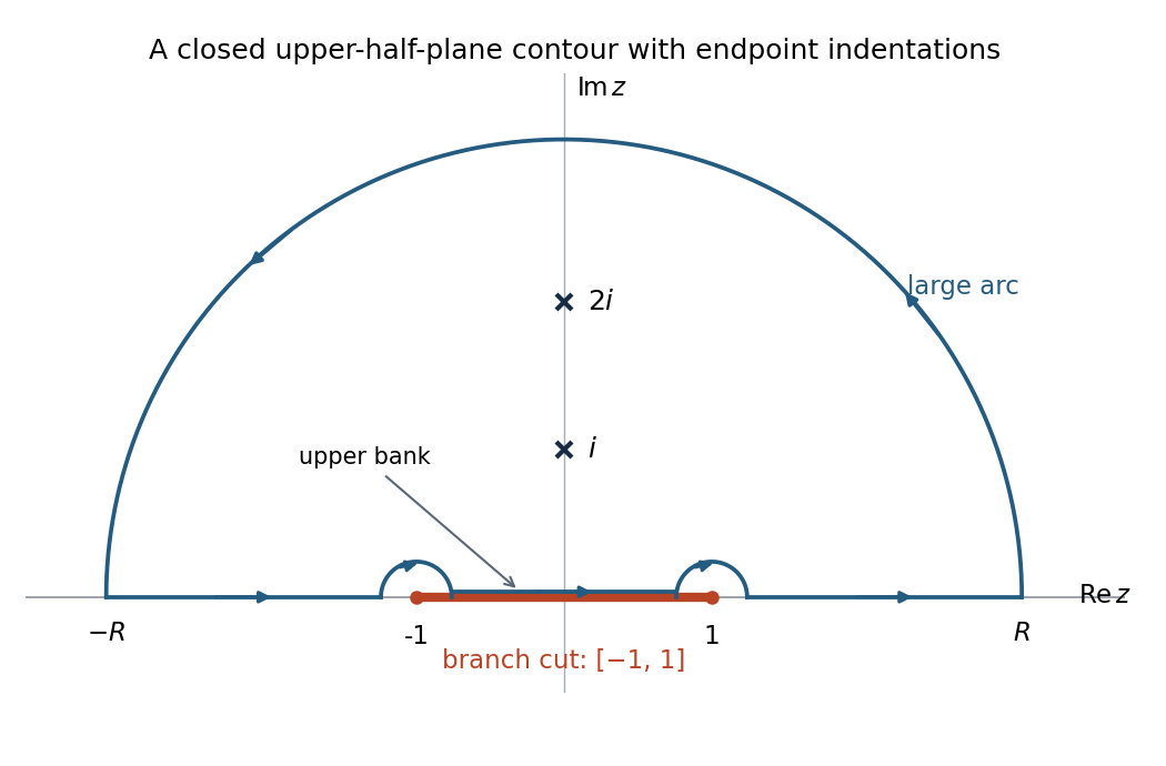
Upper-half-plane contour, clockwise endpoint indentations, and the two enclosed poles; indentation sizes are exaggerated
. Details. The contributions can be controlled separately. Since , the large arc contributes . Near either branch point, , so an arc of length contributes . On the upper bank of ,which is odd in , so its integral is zero. On the exterior real intervals , while the rational numerator is odd. Hence and the two exterior contributions sum to .
Pinned article: Introduction to the OurBigBook Project
Welcome to the OurBigBook Project! Our goal is to create the perfect publishing platform for STEM subjects, and get university-level students to write the best free STEM tutorials ever.
Everyone is welcome to create an account and play with the site: ourbigbook.com/go/register. We belive that students themselves can write amazing tutorials, but teachers are welcome too. You can write about anything you want, it doesn't have to be STEM or even educational. Silly test content is very welcome and you won't be penalized in any way. Just keep it legal!
Intro to OurBigBook
. Source. We have two killer features:
- topics: topics group articles by different users with the same title, e.g. here is the topic for the "Fundamental Theorem of Calculus" ourbigbook.com/go/topic/fundamental-theorem-of-calculusArticles of different users are sorted by upvote within each article page. This feature is a bit like:
- a Wikipedia where each user can have their own version of each article
- a Q&A website like Stack Overflow, where multiple people can give their views on a given topic, and the best ones are sorted by upvote. Except you don't need to wait for someone to ask first, and any topic goes, no matter how narrow or broad
This feature makes it possible for readers to find better explanations of any topic created by other writers. And it allows writers to create an explanation in a place that readers might actually find it.
Figure 1. Screenshot of the "Derivative" topic page. View it live at: ourbigbook.com/go/topic/derivativeVideo 2. OurBigBook Web topics demo. Source. - local editing: you can store all your personal knowledge base content locally in a plaintext markup format that can be edited locally and published either:This way you can be sure that even if OurBigBook.com were to go down one day (which we have no plans to do as it is quite cheap to host!), your content will still be perfectly readable as a static site.
- to OurBigBook.com to get awesome multi-user features like topics and likes
- as HTML files to a static website, which you can host yourself for free on many external providers like GitHub Pages, and remain in full control

Figure 2. You can publish local OurBigBook lightweight markup files to either OurBigBook.com or as a static website.
Figure 3. Visual Studio Code extension installation.
Figure 5. . You can also edit articles on the Web editor without installing anything locally. Video 3. Edit locally and publish demo. Source. This shows editing OurBigBook Markup and publishing it using the Visual Studio Code extension. 
- Infinitely deep tables of contents:




All our software is open source and hosted at: github.com/ourbigbook/ourbigbook
Further documentation can be found at: docs.ourbigbook.com
Feel free to reach our to us for any help or suggestions: docs.ourbigbook.com/#contact