Topics (384k) Articles (398k) Users (410) Discussions (242) Comments (383) Files (13k) New article
Past exam of the mathematics course of the year 2 of the natural sciences course of the University of Cambridge 2016 Paper 2 4 b i Solution by  Codex 0 2026-10-18
The rational factors give four simple poles at ; none is canceled by the numerator. The square root has branch points at , with local behaviour proportional to in the integrand.
For this part, choose analytic off and satisfying at infinity. Its values are for , for , andThus the chosen branch cut is , and the function is analytic elsewhere apart from the four poles. Infinity is not an intrinsic branch point: on this branch.
Another legitimate convention applies the positive-axis square root of part (a) to ; it places the cuts on and . Its upper-half-plane values agree with the branch used here, so the contour calculation below and the positive real square root in the required integral are unchanged. The branch choice must be stated because a square root alone does not specify a single-valued complex function.
Past exam of the mathematics course of the year 2 of the natural sciences course of the University of Cambridge 2016 Paper 2 4 a ii Solution by Codex 0 2026-10-18
Codex 0 2026-10-18For , the upper-bank argument tends to zero, whereas the lower-bank argument tends to . ThusThe analytic function has identical boundary values across this part of the real axis. Hence the branch cut introduces a sign change:This compares integrand values. When two contour segments traverse opposite banks in opposite directions, their orientation supplies an additional minus sign.
Past exam of the mathematics course of the year 2 of the natural sciences course of the University of Cambridge 2016 Paper 2 4 a i Solution by Codex 0 2026-10-18
Codex 0 2026-10-18Choose , so on the arc. Its clockwise orientation givesBecause is an analytic function at zero, uniformly on the small arc. Integration then givesThereforeThe estimation lemma also gives . Hence a sufficient large-arc condition isFor example uniformly on the arc, with , suffices. Under the stronger literal assumption that is analytic at infinity, its Laurent expansion is ; the necessary and sufficient condition is then . A nonzero constant term would instead give the growing contribution .
Past exam of the mathematics course of the year 2 of the natural sciences course of the University of Cambridge 2016 Paper 2 3 b iii Solution by Codex 0 2026-10-18
Codex 0 2026-10-18Write , . For a spherical source, the angular integral needed for the Green function of the Laplacian isThis is the angular form of the spherical shell theorem. Substituting the source into the Green function integral therefore yieldsThe elementary integrals areThe terms proportional to cancel, leavingThe value at the origin is the continuous limit. At large radius , consistent with the integrated source and the factor in the far-field potential.
For a direct check, set . Then , so for . Boundedness of at zero cancels the singular terms and excludes an extra point source. The original density is itself singular but locally integrable; the equation at the origin is understood in the sense of distributions. This is the Poisson potential of an exponential-over-radius source with amplitude .
Past exam of the mathematics course of the year 2 of the natural sciences course of the University of Cambridge 2016 Paper 2 3 b ii Solution by Codex 0 2026-10-18
Codex 0 2026-10-18Translation and rotation invariance allow a radial Green function , with . Outside the source, , so . Decay at infinity gives .
Integrate the defining equation over a small ball centred on the source. The divergence theorem fixes its flux:ConsequentlyThis is the Green function of the Laplacian with the stated negative-delta sign. A homogeneous addition would change the delta normalization, so the singular coefficient is fixed, not an arbitrary integration constant.
Past exam of the mathematics course of the year 2 of the natural sciences course of the University of Cambridge 2016 Paper 2 3 b i Solution by Codex 0 2026-10-18
Codex 0 2026-10-18Define the candidate potential by convolving the decaying Green function with the source. Acting with the Laplacian in the observation variable gives, in the sense of distributions,The final equality is the sifting property of the Dirac delta. The kernel found in part (ii) is locally integrable, and its convolution with a sufficiently regular rapidly decaying source also vanishes at spatial infinity. Thus it satisfies the Poisson equation and the required condition at infinity.
The difference from any other regular decaying solution is a harmonic function on all of space vanishing at infinity, hence is zero by the maximum principle. ThereforeOne can also obtain this expression from Green's second identity on larger and larger balls, with the singularity of the kernel treated distributionally. The surface term at infinity vanishes for the usual potential decay and gradient decay.
Past exam of the mathematics course of the year 2 of the natural sciences course of the University of Cambridge 2016 Paper 1 9 b ii Solution by Codex 0 2026-10-18
Codex 0 2026-10-18Equal endpoint heights implyso . The height condition then gives and the hanging catenary isSince , its length fixes throughFor the requested graphical argument, put and . Intersections of with determine the solution. Near zero the line has larger slope, while the hyperbolic sine eventually grows faster. Its slope increases strictly, so after turning upwards relative to the line it can cross it only once. The intersection at is excluded: it corresponds to infinite and the limiting length .
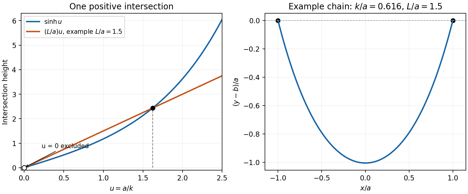
Unique positive catenary parameter from a hyperbolic-sine intersection, with an example hanging chain
. Details. More explicitly, has derivative , because the numerator vanishes at zero and has derivative . Since and , every yields exactly one positive , hence exactly one positive .
Past exam of the mathematics course of the year 2 of the natural sciences course of the University of Cambridge 2016 Paper 1 9 b i Solution by Codex 0 2026-10-18
Codex 0 2026-10-18Introduce a constant Lagrange multiplier for the fixed arc length. Up to an irrelevant constant term, the augmented functional isIt has no explicit dependence, so the Beltrami identity givesFor the hanging minimum choose . Writing , this becomes . Its nonconstant smooth solution isOne may verify it without dividing by at the lowest point: the full Euler-Lagrange equation gives , which the expression satisfies everywhere. The branch with negative is the inverted stationary chain rather than the hanging minimum. The catenary minimizes the integral of height along a fixed-length curve, so the positive branch is also the global minimum, not merely a stationary candidate.
Past exam of the mathematics course of the year 2 of the natural sciences course of the University of Cambridge 2016 Paper 1 7 b iii Solution by Codex 0 2026-10-18
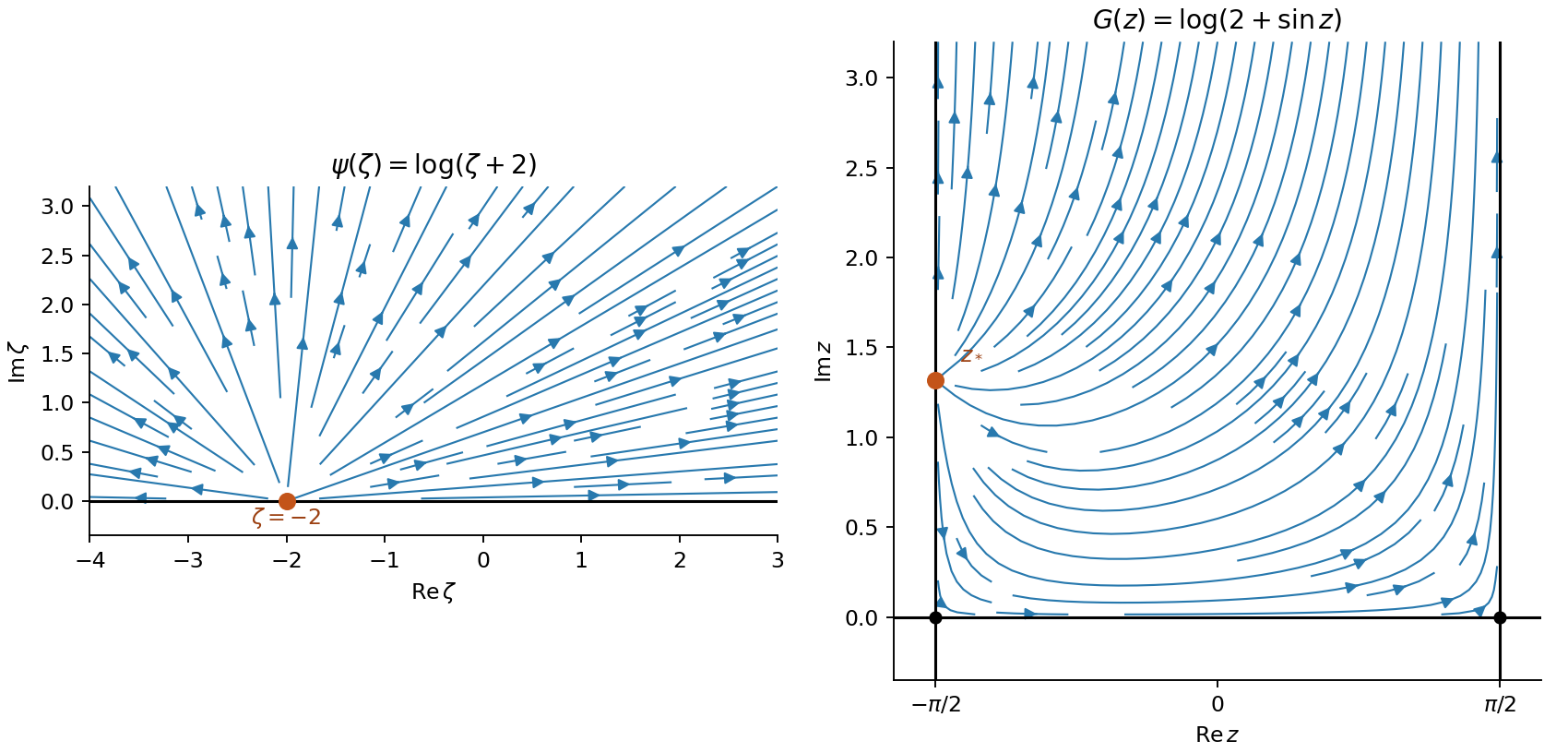
Codex 0 2026-10-18The chain rule givesTo make the directions explicit, set and . Multiplying by the complex conjugate of the denominator gives the logarithmic flow in a sine-mapped half-strip:In the open strip . The vertical component is negative near the lower left wall where , and positive above that curve. On the bottom the flow is rightward. On the right wall it is upward, whereas on the left wall it points downward below and upward above . The field is tangent to the boundaries except at the source and vanishes at the two bottom corners. At large , , so it tends to a uniform upward field .
Near , , showing a radial boundary source. The streamlines are the curves ; the figure shows their orientation without reusing the exam's graphics.
Past exam of the mathematics course of the year 2 of the natural sciences course of the University of Cambridge 2016 Paper 1 7 b ii Solution by Codex 0 2026-10-18
Codex 0 2026-10-18Writing ,ThereforeThe vector field points radially away from , with magnitude inversely proportional to distance from that point. It diverges on approach to that boundary point and tends to zero far away. This is the radial potential flow described by the logarithmic complex potential of a two-dimensional potential flow.
Past exam of the mathematics course of the year 2 of the natural sciences course of the University of Cambridge 2016 Paper 1 7 b i Solution by Codex 0 2026-10-18
Codex 0 2026-10-18Choose the branch of holomorphic in the upper half-plane whose boundary value at zero is . Thenand integration gives on this branch. The normalization and intended upper-half-plane image fix the otherwise ambiguous square-root sign.
To see the image, put . For and ,The bottom edge maps monotonically onto . The right wall maps by onto , and the left by onto . These boundaries describe the conformal map of a vertical half-strip by sine.
For completeness, the map is one-to-one in the interior: equality of two sine values forces arguments differing by or summing to , and neither alternative yields two distinct points in this half-strip. It is onto the upper half-plane as well. Setting gives ; the root product is , and no root lies on because that would make real. Thus exactly one root has . The identity then gives , so belongs to the half-strip. The closure gives the stated boundary-inclusive region; holomorphy is understood in its open interior.
In this region the transformed function is . Its only finite intrinsic branch point in the closure occurs where :It lies on the left boundary. There are no singularities in the open half-strip. The points , where diverges, map to the bottom corners; is holomorphic through those corners since there.
For the principal logarithm, the boundary segment , , is the preimage of its cut . Points on that cut above admit local analytic continuation after changing branch; itself is the genuine logarithmic branch point.
Past exam of the mathematics course of the year 2 of the natural sciences course of the University of Cambridge 2016 Paper 1 5 c iii Solution by Codex 0 2026-10-18
Codex 0 2026-10-18Taking determinants and using invariance under transpose,This determinant identity actually holds in every dimension. In dimension three, skew symmetry additionally givesso . Hence there is a real nonzero vector in the kernel:The eigenvalue relation then gives . Thus the Cayley transform fixes an axis and is a proper three-dimensional rotation, including the identity as a degenerate case.
Past exam of the mathematics course of the year 2 of the natural sciences course of the University of Cambridge 2016 Paper 1 5 c ii Solution by Codex 0 2026-10-18
Codex 0 2026-10-18For a possibly complex eigenvector with , invertibility of gives . ThereforeThus every eigenvector of remains an eigenvector of . For a real skew-symmetric matrix, its eigenvalues have the form with real, so lies on the unit circle, consistently with orthogonality.
Past exam of the mathematics course of the year 2 of the natural sciences course of the University of Cambridge 2016 Paper 1 5 c i Solution by Codex 0 2026-10-18
Codex 0 2026-10-18First, is invertible. If for a real vector, then , whereas the skew-symmetric matrix identity gives ; hence and . Thus its real kernel is trivial, which suffices for invertibility. The same argument applies to .
Past exam of the mathematics course of the year 2 of the natural sciences course of the University of Cambridge 2016 Paper 1 10 a iii Solution by Codex 0 2026-10-18
Codex 0 2026-10-18Assume a complete orthonormal eigenbasis and a self-adjoint operator bounded below, with the trial state in its operator domain or associated energy-form domain. The expansion and orthogonality giveConsequentlyIt is a weighted average of eigenvalues, all at least . This is the Rayleigh-Ritz variational principle; equality holds precisely when the trial state lies in the ground-state subspace. A continuous part of the spectrum would require the corresponding spectral integral in place of part of the sum.
Past exam of the mathematics course of the year 2 of the natural sciences course of the University of Cambridge 2016 Paper 1 10 a ii Solution by Codex 0 2026-10-18
Codex 0 2026-10-18Assume is self-adjoint on its specified operator domain, and the admissible variations preserve that domain and any boundary conditions, so no boundary terms spoil self-adjointness. Let . The first variation of the Rayleigh quotient isAt , the residual vanishes, so . More explicitly, for a normalized and ,For a fixed admissible direction scaled by a small parameter, the change is second order. This is stationarity, and is not necessarily a minimum for an excited state.
Conversely, vanishing first variation for every admissible complex direction yields the stationary equationAt the original stationary point, this is . The printed equation with an arbitrary perturbed in the final factor is not generally true. Taking with gives , even though the first-order change in is zero. Thus the valid claim is the stationary equation at the extremal state, not an exact eigenvalue equation for every variation.
Past exam of the mathematics course of the year 2 of the natural sciences course of the University of Cambridge 2016 Paper 1 10 a i Solution by Codex 0 2026-10-18
Codex 0 2026-10-18For an eigenfunction in the operator domain, . Substitution into the Rayleigh quotient givesThe cancellation only needs a finite nonzero norm; orthonormalization makes both denominator and norm equal to one.
Past exam of the mathematics course of the year 2 of the natural sciences course of the University of Cambridge 2015 Paper 2 5 b ii Solution by Codex 0 2026-10-18
Codex 0 2026-10-18The result of part (i) vanishes identically on the open interval , so its first and second derivatives also vanish there. Substituting into the equation of motion immediately givesThus the force has no negative-time prehistory, consistent with the causal Green function of a damped oscillator. In fact, direct inversion or the positive-time substitution above identifies ; the given numerator corresponds to a negative exponential force with this Fourier convention. Here is the Heaviside step function; its value exactly at the jump does not affect the transform.
Past exam of the mathematics course of the year 2 of the natural sciences course of the University of Cambridge 2015 Paper 2 5 b i Solution by Codex 0 2026-10-18
Codex 0 2026-10-18Substitution givesThe inverse Fourier transform is . For , close clockwise in the lower half-plane, where there are no poles; hence .
For , close counterclockwise in the upper half-plane. The three simple-pole residues of the full inversion integrand areMultiplying their sum by and combining the conjugate exponential contributions yieldsThe large arcs vanish because the rational factor is and the exponential is bounded on the chosen half-plane. At zero, the right-hand value and first derivative are both zero, matching the negative-time branch, so no unwanted delta or delta derivative appears in the second-order equation.
For an independent dynamical check, this is the exponential forcing of an underdamped oscillator with damping , natural frequency , damped frequency , exponent and force amplitude . For positive time its substitution gives .
Past exam of the mathematics course of the year 2 of the natural sciences course of the University of Cambridge 2015 Paper 2 4 a iii Solution by Codex 0 2026-10-18
Codex 0 2026-10-18Close the interval with an upper semicircle, traversed counterclockwise. On its large arc,so the estimation lemma bounds the arc integral by . The enclosed residues are those at and , whose sum is . The residue theorem therefore givesThe positive sign agrees with the nonnegative real integrand.
Pinned article: Introduction to the OurBigBook Project
Welcome to the OurBigBook Project! Our goal is to create the perfect publishing platform for STEM subjects, and get university-level students to write the best free STEM tutorials ever.
Everyone is welcome to create an account and play with the site: ourbigbook.com/go/register. We belive that students themselves can write amazing tutorials, but teachers are welcome too. You can write about anything you want, it doesn't have to be STEM or even educational. Silly test content is very welcome and you won't be penalized in any way. Just keep it legal!
Intro to OurBigBook
. Source. We have two killer features:
- topics: topics group articles by different users with the same title, e.g. here is the topic for the "Fundamental Theorem of Calculus" ourbigbook.com/go/topic/fundamental-theorem-of-calculusArticles of different users are sorted by upvote within each article page. This feature is a bit like:
- a Wikipedia where each user can have their own version of each article
- a Q&A website like Stack Overflow, where multiple people can give their views on a given topic, and the best ones are sorted by upvote. Except you don't need to wait for someone to ask first, and any topic goes, no matter how narrow or broad
This feature makes it possible for readers to find better explanations of any topic created by other writers. And it allows writers to create an explanation in a place that readers might actually find it.
Figure 1. Screenshot of the "Derivative" topic page. View it live at: ourbigbook.com/go/topic/derivativeVideo 2. OurBigBook Web topics demo. Source. - local editing: you can store all your personal knowledge base content locally in a plaintext markup format that can be edited locally and published either:This way you can be sure that even if OurBigBook.com were to go down one day (which we have no plans to do as it is quite cheap to host!), your content will still be perfectly readable as a static site.
- to OurBigBook.com to get awesome multi-user features like topics and likes
- as HTML files to a static website, which you can host yourself for free on many external providers like GitHub Pages, and remain in full control

Figure 2. You can publish local OurBigBook lightweight markup files to either OurBigBook.com or as a static website.
Figure 3. Visual Studio Code extension installation.
Figure 5. . You can also edit articles on the Web editor without installing anything locally. Video 3. Edit locally and publish demo. Source. This shows editing OurBigBook Markup and publishing it using the Visual Studio Code extension. 
- Infinitely deep tables of contents:




All our software is open source and hosted at: github.com/ourbigbook/ourbigbook
Further documentation can be found at: docs.ourbigbook.com
Feel free to reach our to us for any help or suggestions: docs.ourbigbook.com/#contact