For positive integer $k$, the equivalence is the bounded invariant norm characterization of cusp forms. The three conditions below work together: meromorphicity and the bound remove interior poles; the transformation law produces a periodic local function at every modular cusp; the same bound makes that function tend to zero at the modular cusp. Conversely a cusp form has exponentially decaying Fourier expansions of a modular form, and finitely many compact core regions control its invariant norm everywhere. These implications are proved under the corresponding labelled items.

Without a positive-weight convention, weight zero is a genuine exception. The function $f=1$ satisfies all three printed conditions at $k=0$ for every congruence subgroup, but is not a cusp form. Indeed a weight-zero cusp form would descend to a holomorphic function on the compact curve $X(\Gamma )$ and hence be constant, and vanishing at a modular cusp would make it zero. Thus the literal unrestricted claim needs the qualification $k>0$.

If negative integer weights are included, both sides contain only the zero function. To check the bounded side, each modular cusp translate has at most power growth in $y$, hence at most a power of $\log (1/|q_h|)$. For a negative Laurent coefficient of order $m$, Cauchy's coefficient estimate bounds its absolute value by $C{r}^m(\log (1/r){)}^{|k|/2}\to 0$, so there is no negative coefficient and every modular cusp is holomorphic. If such a nonzero negative-weight form existed, the product of its slash translates over $\Gamma \backslash S{L}_2(\mathbb{Z})$ would be a nonzero holomorphic level-one modular form of negative weight. Right multiplication permutes the translates, and all modular cusp factors are bounded, so that product really is a level-one form. Its existence contradicts the valence formula. This also excludes negative-weight modular cusp forms. The nonzero counterexample is specifically weight zero.

Use the comultiplication $\Delta E=E\otimes K+1\otimes E$, $\Delta F=F\otimes 1+K^{-1}\otimes F$, $\Delta K=K\otimes K$ of the quantum enveloping algebra of sl2. Choose a basis $u_0,u_1$ for $V_{1,1}$ with $F{u}_0=u_1$, $E{u}_1=u_0$, and $K{u}_i=q^{1-2i}{u}_i$. Choose a basis $w_0,w_1,w_2$ for $V_{1,2}$ withand all terminal raising or lowering actions zero. This is one of the corrected bases from part (a).

In the tensor product of modules, putThe vector $z_0$ is killed by $E$ and has $K$ eigenvalue $q^3$. Direct application of the comultiplication givesand the string formula gives $E{z}_1=[3]z_0$, $E{z}_2=[2]z_1$, $E{z}_3=z_2$. Also $K{z}_i=q^{3-2i}{z}_i$. Thus $W_3=⟨z_0,z_1,z_2,z_3⟩$ is a submodule isomorphic to $V_{1,3}$.

The other highest vector and its lowered partner areIndeed $E{h}_0=([2]q^2-q^2[2])u_0\otimes w_0=0$, $K{h}_0=q{h}_0$, $K{h}_1=q^{-1}{h}_1$, $E{h}_1=h_0$ and $F{h}_1=0$. Therefore $W_1=⟨h_0,h_1⟩$ is a submodule isomorphic to $V_{1,1}$.

To verify that this is a direct sum, in the $q$ weight space the determinant of the coefficients of $z_1,h_0$ is $-q^2-q^{-1}[2]=-[3]\ne 0$. In the $q^{-1}$ weight space, the coefficient determinant of $z_2,h_1$ is $-q[2]-q^{-2}=-[3]\ne 0$. The extreme weight spaces are spanned by $z_0,z_3$. Hence these six vectors form a basis of the entire tensor product of modules. Each summand is a simple module: projecting a nonzero vector onto one of its distinct $K$ weight spaces and applying the nonzero raising and lowering coefficients recovers its entire basis. Consequently

Use the Fourier convention $\hat{f}(\xi )={\int }_{{\mathbb{R}}^3}{e}^{-ix\cdot \xi }f(x)dx$, with inverse $(2\pi {)}^{-3}\int e^{ix\cdot \xi }\hat{f}(\xi )d\xi$. For a tempered distribution $T$, define its Fourier transform by duality:The Fourier transform maps the Schwartz space continuously onto itself, making the right side a continuous linear functional there. The use of the same negative exponential in the test-function transform is consistent with bilinear distributional pairing; other unitary or sign conventions change the normalization accordingly.

The interval indicator has transformwith continuous value $2b$ at $k=0$. By the convolution theorem, $h=f\ast g$ has transform $4a\sin (bk)/[k(a^2+k^2)]$. Fourier inversion therefore expresses the requested integral asFor $x>b$, $|x-y|=x-y$, so $h(x)=2e^{-ax}\sinh (ab)/a$. Symmetry gives the same expression with $|x|$ for $x<-b$. For $|x|\le b$, splitting the integral at $y=x$ givesConsequently the value for every real $x$ isThe two expressions agree at $x=\pm b$. This is the exponential kernel convolved with an interval indicator. The spectral integral is absolutely convergent: its apparent singularity at zero is removable, and the tail decays as $O(|k{|}^{-3})$.

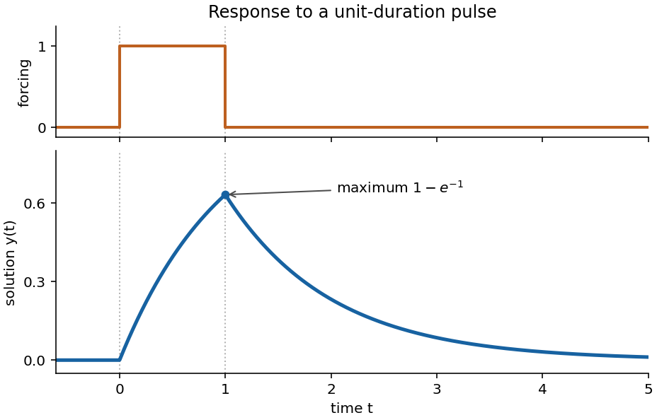
The forcing is a unit pulse on $0<t<1$. For $t<0$, the homogeneous equation and continuity with $y(0)=0$ give $y=0$. On $0<t<1$, integration with $y(0)=0$ gives $y=1-e^{-t}$. At the end of the pulse its value is $1-e^{-1}$, and the subsequent homogeneous decay must start at that value. ThusEquivalently it is the difference of two translated step responses, $(1-e^{-t})H(t)-(1-e^{-(t-1)})H(t-1)$. The solution is continuous, rises concavely to its maximum $1-e^{-1}$ at $t=1$, and then decays exponentially to zero. Its derivative has jumps at the pulse edges; those are permitted because the right-hand side has step discontinuities.

The sphere-plane intersection is governed by the orthogonal projection of the sphere's centre onto the plane. Since $\mathbf{n}$ has unit length, let $h=p-\mathbf{n}\cdot \mathbf{c}$, the signed distance from $\mathbf{c}$ to the plane along $\mathbf{n}$. The following parts determine the centre and radius and retain this sign; the radii alone cannot distinguish the two possible sides of the oriented plane.

First resolve the orientation sign in quadrant harmonic spectral inversion. The printed spectral definitions traverse the physical boundary clockwise, whereas both reconstruction rays run outward from zero. Integrating first in $k$ gives the kernel $i/(z-w)$. The resulting clockwise Cauchy integral is the negative of the desired holomorphic function. Thus, with exactly the spectral definitions used above, the consistent reconstruction isThe printed plus sign would reconstruct $-q_z$. For a concrete nonzero example, $q(z)=-2\mathrm{Re}[(1+i)/(z+1+i)]$ is real, harmonic, smooth on the closed quadrant and decays along both axes. With ${\beta }_1={\beta }_2=0$, it has $h_1(0)=h_2(0)=1$ and $q_z=(1+i)/(z+1+i{)}^2$. The printed orientation returns the negative of this derivative, so the issue persists even under the stated corner condition.

Let $a=\frac{1}{2}{e}^{-i{\beta }_1-i\gamma }$. In the expressions from the preceding part, the coefficient of $\Phi$ on the imaginary ray is $a$, and the coefficient on the real ray is $-a{e}^{4i\gamma }$. For each of the three allowed sums, $e^{4i\gamma }=1$. The unknown part is therefore proportional toIndeed, close the first spectral quadrant. For $z=x+iy$ with $x,y>0$, $|e^{ikz}|=e^{-(x\mathrm{Im}k+y\mathrm{Re}k)}$, so the large-arc contribution vanishes for bounded $\Phi$. The Cauchy integral theorem proves the equality and eliminates the single unknown function.

Substituting only the known pieces leavesThis already determines the answer from $h_1,h_2$ alone. Evaluating the elementary ray kernels gives the more direct rational-angle oblique derivative problem on a quadrant formulaNo denominator vanishes for an interior point of the first quadrant.

For explicit formulas in the three cases, defineCombining the paired fractions and using ${\beta }_2=\gamma -{\beta }_1$ yields

There is also a necessary corner compatibility for collinear oblique derivative data. When $\gamma =\pi /2$, the two prescribed derivative directions are opposites, so a continuous corner gradient requires $h_2(0)=-h_1(0)$. Together with the stipulated equality, this forces $h_1(0)=h_2(0)=0$ in that case. Existence was assumed, so admissible data must satisfy this additional consequence. Smoothness at the corner and decay at infinity also exclude the homogeneous corner ambiguity in a quadrant Laplace problem; no extra singular or growing term is permitted in the boxed reconstruction.

Since $q$ is harmonic, $q_z$ is holomorphic and the one-form $e^{-ikz}{q}_{z}dz$ is closed. Closing the physical quadrant at infinity gives the global relationIn this third spectral quadrant the exponential decays on both boundary axes. Set $\gamma ={\beta }_1+{\beta }_2$. The relation becomes

All four boundary functions are real. Consequently their transforms obeyand the same identities for $J_1,J_2$. Complex conjugation of the global relation therefore gives its upper-left consequenceIntroduce just one unknown function,It is holomorphic in the upper half-plane. Under the transform-admissible decay assumptions, $|\Phi (k)|\le {\int }_0^{\infty }(|h_2|+|j_2|)dx$, so it is bounded there.

For $k$ on the positive real ray, use both consequences of the global relation at $-k$. Adding them removes $J_1(-k)$ and givesFor $k$ on the positive imaginary ray, use the upper-left relation and $H_2(-k)+i{J}_2(-k)=2H_2(-k)-\Phi (k)$. The resulting single-function spectral elimination for a rational-angle quadrant isBoundary limits from the appropriate transform domains are understood. Every remaining unknown boundary derivative is contained in the one bounded upper-half-plane function $\Phi$.

Let $s_j=\sin {\beta }_j$, $c_j=\cos {\beta }_j$. Inverting the two orthogonal derivative systems gives, on the vertical axis,and, on the horizontal axis,Using the Wirtinger derivative $q_z=(q_x-i{q}_y)/2$, these become

Define the appropriate boundary transforms byThe first pair is holomorphic for $\mathrm{Re}k<0$; the second pair consists of Half-range Fourier transforms, holomorphic for $\mathrm{Im}k<0$. Parametrizing the vertical boundary by $z=iy$ gives $dz=idy$, which must be retained. Substitution yields the quarter-plane oblique boundary spectral functions:Their signs follow from the stated clockwise boundary orientations: upward on the left and inward on the bottom.

For fixed cosmological density parameters, the redshift drift has the form $\dot{z}=H_{0}F(z)$. Multiplying the Hubble constant changes the vertical scale of all three sketches but leaves their zeros unchanged. Thus the drift-zero redshift is independent of $H_0$ at fixed density fractions. Every model has the trivial $z=0$ zero; only the specified mixed model has a further positive zero, $z_{\ast }\simeq 2.089$. If instead physical matter and vacuum densities are held fixed while $H_0$ changes, their density fractions change too, so that is a different family of models.

We first derive the recurrence needed for the partition of unity. Denote an order-$r$ partition-normalized spline by $N_{i,r}$. For $r\ge 2$, set $h_t(u)=(u-t{)}_{+}^{r-2}$, so $(u-t)h_t(u)=(u-t{)}_{+}^{r-1}$. The elementary product identities for divided differences areThey follow from the Leibniz rule for divided differences because the divided differences of the linear factor vanish above first order. Use the first identity on $t_i,\dots ,t_{i+r-1}$ and the second on $t_{i+1},\dots ,t_{i+r}$. Subtracting cancels the common middle-block term. The defining divided-difference recurrence for $N_{i,r}$ then givesThis is the Cox-de Boor recurrence, derived here from the specified normalization rather than assumed as a partition theorem.

Extend the distinct knot sequence in both directions to a strictly increasing sequence $(t_i{)}_{i\in \mathbb{Z}}$ tending to $\pm \infty$. For order one, $N_{i,1}=1_{[t_i,t_{i+1})}$, so the full sum equals one. All higher-order splines are supported on $[t_i,t_{i+r}]$, making the following sums locally finite. Reindexing the second term of the recurrence yieldsInduction proves that the full sum is one for every order. The same recurrence gives nonnegativity: each coefficient is nonnegative wherever its associated lower-order spline is nonzero. Removing splines therefore gives the subpartition of unity for B-splines on the whole line.

For $t_k<t<t_{n+1}$, a spline with index $i\le 0$ ends no later than $t_k$, and one with $i\ge n+1$ starts no earlier than $t_{n+1}$. They all vanish, leaving exactly the indices $1,\dots ,n$. For $k\ge 2$ the splines are continuous and vanish at their support endpoints, so the equality extends to the closed basic knot interval:If order one is allowed, the standard half-open indicator convention gives equality on $[t_1,t_{n+1})$; to include its final endpoint literally, assign the left-limit value there. This harmless endpoint convention does not change integrals or $L^{\infty }$ norms. For the continuous splines of order at least two no such convention is necessary.

With spatial flatness, the scalar as the only source, and $M_{\mathrm{Pl}}=(8\pi G{)}^{-1/2}$, the Friedmann equation isThe scalar equation gives $\dot{\rho }=\dot{\varphi }(\ddot{\varphi }+V_{,\varphi })=-3H{\dot{\varphi }}^2$, which is the energy-conservation equation $\dot{\rho }+3H(\rho +P)=0$. Differentiating the Friedmann equation on the expanding branch yields $6M_{\mathrm{Pl}}^{2}H\dot{H}=-3H{\dot{\varphi }}^2$, so $\dot{H}=-{\dot{\varphi }}^2/(2M_{\mathrm{Pl}}^2)$. Combining this with $\ddot{a}/a=H^2+\dot{H}$ gives the Friedmann acceleration equation:Thus cosmic inflation occurs exactly when $V(\varphi )>{\dot{\varphi }}^2$ in this canonical scalar model. Equivalently $P<-\rho /3$, or the first Hubble slow-roll parameter ${ϵ}_H=-\dot{H}/H^2$ is smaller than one.

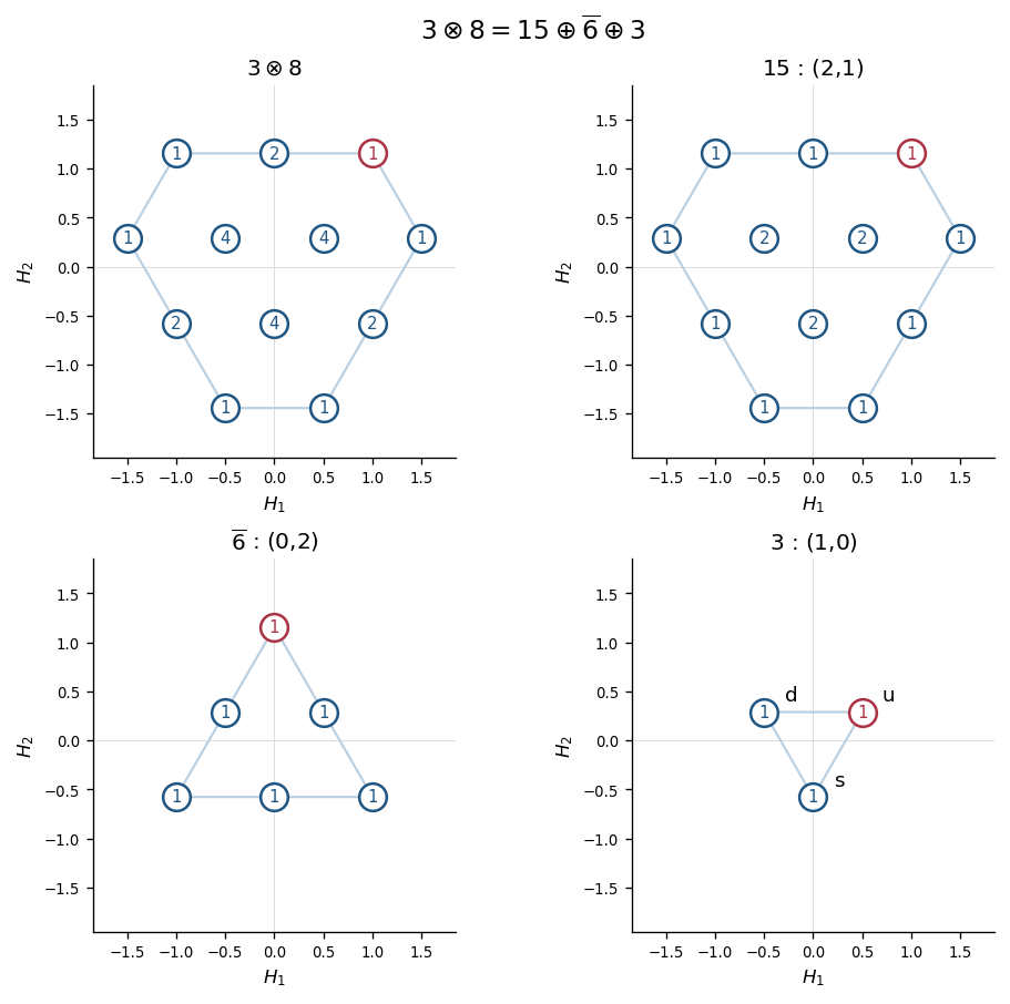
Construct the tensor-product weight diagram by placing one octet diagram at each triplet representation weight $u,d,s$ and adding multiplicities where the shifted diagrams overlap. Its highest weight isso remove the $(2,1)$ diagram by highest-weight character subtraction. Its unequal-sided hexagon has nine boundary representation weights of multiplicity one and three interior representation weights of multiplicity two, giving dimension $15$.

To see the remainder explicitly, measure diagram coordinates by $(a,b)=(2h_1,2\sqrt{3}{h}_2)$. After subtracting this $15$, the residual representation weights areThe next highest weight is $(h_1,h_2)=(0,2/\sqrt{3})=2{\omega }_2$, with Dynkin labels $(0,2)$. The conjugate sextet $\overline{6}$ is a triangular weight diagram containing each of these six representation weights once. Subtracting it leaves $(1,1),(-1,1),(0,-2)$ once each in the integer coordinates: precisely the triplet. The SU(3) triplet-octet decomposition is thereforeThe dimensions add to $15+6+3=24$, and the figure below verifies the equality at every representation weight, including overlapping interior representation weights.

For the Metropolis–Hastings algorithm, start at a state $\theta$ with positive target density, propose ${\theta }^{\prime }$ from $q({\theta }^{\prime }\mid \theta )$, and generate an independent uniform draw. Accept the proposal with probabilityOn rejection retain $\theta$, including repeated states in the chain; removing repeats would generally change its stationary law. The accepted-flow density satisfieswhich is symmetric in its two states. This proves detailed balance and hence invariance of the target distribution, including the holding probabilities on the diagonal. Unknown common normalization constants cancel in the ratio. Invariance alone does not establish convergence from arbitrary initial states. Choosing proposals that yield a positive Harris recurrent Markov chain with aperiodicity supplies the usual convergence guarantee, and the resulting sample is dependent. Use burn-in and account for autocorrelation when assessing Monte Carlo precision.