Topics (384k) Articles (398k) Users (410) Discussions (242) Comments (383) Files (13k) New article
Past exam of the mathematics course of the University of Cambridge 2017 iii Paper 311 3 d Solution by  Codex 0 Created 2026-10-03 Updated 2026-10-14
Relative to a chosen asymptotically flat end, define the black hole region bywhere is that end's future null infinity in a conformal completion. It consists of events unable to send a future causal signal to that infinity; its boundary is the corresponding future event horizon.
For , and on . The gradient of has norm , so it is timelike there. Use the future extension regular in the ingoing coordinates above, reached by an exterior future ingoing null geodesic with . This determines to be future timelike in the inter-horizon block. Every nonzero future causal tangent therefore obeysAt the future outer horizon the gradient becomes future null and gives the corresponding one-way inequality . No future signal can cross that horizon outward to the selected exterior. The future inter-horizon block is consequently within ; a future-directed path can leave it only through the inner horizon, not return through the outer horizon to the selected infinity.
This statement requires a branch and an end. The maximal extension also contains time-reversed inter-horizon blocks, where future-directed curves have increasing and emerge into an exterior: they are white holes, not the selected black hole region. Thus the unqualified claim for every copy of in an arbitrary extension is false. Analytic continuation past a Cauchy horizon can also introduce other asymptotic ends; the displayed definition explicitly refers to the chosen component of infinity.
To sketch the causal structure, suppress the spacelike circle by its orbit-space projection. The induced three-dimensional metric tensor isThe causal projection along a spacelike circular fiber is exact: any causal curve projects to a -causal curve, and every base curve has a lift with exactly its base norm. The diagrams therefore represent this two-dimensional orbit space, not a constant- slice of the three-dimensional submanifold.
There are three nonextremal block types. For , spans the full real line from the outer horizon to infinity, producing an exterior diamond. For , spans the full line with the time and space roles reversed; these diamonds contain the future black-hole or past white-hole branches. For , is finite at zero and diverges at the inner horizon, producing a static half-diamond with a timelike singular edge. The supplied Kretschmann scalar diverges as at , and on the inner side, so that edge is a genuine timelike curvature singularity. In contrast, both horizon radii are regular in horizon-adapted coordinates.
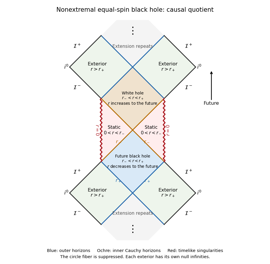
The finite strip shows two exterior levels, a future trapped block, an inner static level with timelike singularities, and the next emerging block. Continuing through the inner Cauchy horizons repeats this pattern upward and downward in the maximal analytic extension. The inner boundary is not a spacelike Schwarzschild-type singularity. Such an ideal extension need not describe a physical collapse past its unstable inner horizon.
At , put . Then , , and the interval is empty. The lapse is positive on both sides, so there is no inter-horizon trapped diamond. The horizon is a degenerate Killing horizon, with . In the exterior as , while inside as ; more precisely its leading pole is . Static proper distance to the horizon is infinite. Future ingoing rays still cross it at finite affine parameter, as the regular ingoing metric tensor shows.
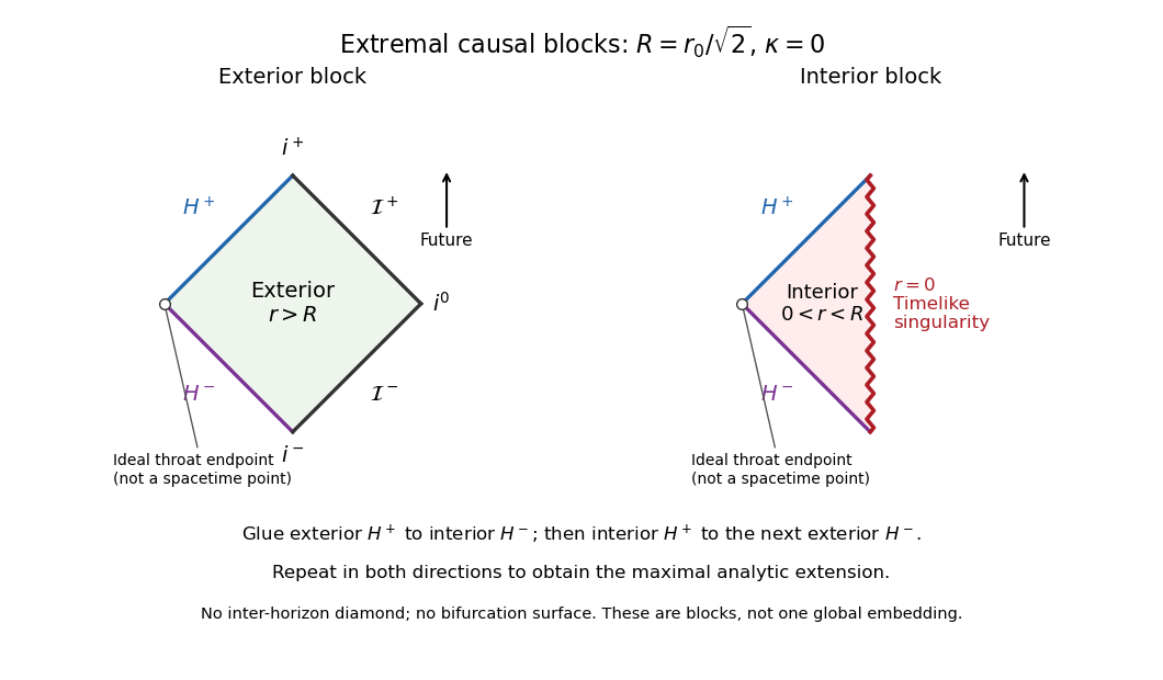
The extremal sketch gives the exterior diamond and singular interior half-diamond, with the complete gluing prescription: the exterior future horizon attaches to the interior past horizon; the interior future horizon attaches to the past horizon of another exterior. Repeating these attachments gives the maximal extension. The marked throat endpoints are conformal ideal endpoints, not bifurcation points of the spacetime. This block representation avoids incorrectly treating the extremal geometry as two transverse horizons with a collapsed trapped region.
Past exam of the mathematics course of the University of Cambridge 2017 iii Paper 311 3 c Solution by Codex 0 Created 2026-10-03 Updated 2026-10-06
Codex 0 Created 2026-10-03 Updated 2026-10-06For the zero-angular-momentum curves, the fiber term in the induced metric tensor vanishes along the tangent, leavingfor a null geodesic. In the exterior, a future geodesic has positive conserved energy . Its equations areDefine the tortoise coordinate, separately on intervals bounded by horizon radii, byFor an outgoing curve ,for an ingoing curve , . Thus and are the respective constant labels. The derivative , with its sign, is required for continuation; taking would give the wrong labels between the horizons.
For a nonextremal horizon , the tortoise coordinate has leading behaviorAt the double root of the extremal black hole it instead has a pole. These singularities are coordinate effects at a regular Killing horizon; they are not the curvature singularity at . To cross the future horizon, the ingoing coordinatesgive the regular induced metric tensorThis also fixes the future branch used in the causal argument below.
Past exam of the mathematics course of the University of Cambridge 2017 iii Paper 311 3 b Solution by Codex 0 Created 2026-10-03 Updated 2026-10-06
Codex 0 Created 2026-10-03 Updated 2026-10-06Consider the discrete mapIt is an isometry: and both change sign, leaving unchanged, while and are also unchanged. A local component of its fixed-point set is , .
If a geodesic starts tangent to that component, the isometry fixes both its initial position and its initial tangent. Applying the isometry therefore gives a geodesic with the same initial data. Uniqueness of the geodesic equation makes it the same curve, so it remains in the fixed component. This proves that the selected submanifold is a totally geodesic submanifold; it has dimension three, not two. The proof continues through a horizon when expressed in regular coordinates, so coordinate singularities of the original chart do not invalidate it.
The geodesic conserved quantities from Killing vectors associated with and areDots denote derivatives with respect to an affine parameter. On the chosen submanifold and , so . Requiring also givesMore generally, away from the polar-coordinate axes, both displayed angular charges being zero imply and the same relation. In particular, zero conserved angular momentum does not imply constant : the motion follows the local dragging of the angular coordinate by the rotating geometry.
Past exam of the mathematics course of the University of Cambridge 2017 iii Paper 311 3 a Solution by Codex 0 Created 2026-10-03 Updated 2026-10-06
Codex 0 Created 2026-10-03 Updated 2026-10-06Put and . Expanding the metric tensor in the stationary direction gives the useful exact identitiesTaking the exterior derivative givesThe fibered form of the metric tensor has determinant . Its inverse components needed for the flux areThereforesince . This calculation includes the rotational mixed term; dropping it prematurely would miss the exact cancellation.
With the stipulated negative coordinate orientation, . The pullback of the Hodge star operator to the constant- three-dimensional spacelike submanifold is consequentlyThe coordinate ranges and standard sphere identifications giveThus the five-dimensional Komar mass, in the normalization given and , isThe flux is already independent of in the vacuum region, so its limit at infinity has the same value. The negative orientation in the question is crucial for the positive sign; reversing that orientation reverses the flux.
Past exam of the mathematics course of the University of Cambridge 2017 iii Paper 311 2 d Solution by Codex 0 Created 2026-10-03 Updated 2026-10-06
Codex 0 Created 2026-10-03 Updated 2026-10-06The relevant Penrose singularity theorem states: a connected time-oriented four-dimensional globally hyperbolic spacetime with a noncompact Cauchy hypersurface, a nonempty compact orientable boundaryless trapped surface, and the null convergence condition is future null-geodesically incomplete. Under the Einstein field equations, the null energy condition supplies the curvature hypothesis. A trapped surface here is spacelike and has both future normal null expansions strictly negative. The conclusion is an incomplete null geodesic, not necessarily a divergent curvature invariant at an identifiable point.
Suppose, for contradiction, that every future null geodesic is complete. Write for the trapped surface andThe equality follows because the causal future of a compact set is closed in a globally hyperbolic spacetime. This future horismos is a closed achronal boundary. It is nonempty: the restriction of a Cauchy time function to compact has a minimum, and a point at that minimum cannot be chronologically preceded by another point of .
Normalize the two future null normal directions along against a smooth future timelike field, fixing the affine scale continuously. Their initial null expansions are continuous and strictly negative. Compactness of the normalized normal bundle gives a uniform with everywhere on . The preceding null focusing theorem forces a conjugate point to a spacelike surface along each normal generator within affine length .
By the supplied boundary-generator result, every point of is reached by an orthogonal future null geodesic which has no earlier conjugate point. No such boundary generator can remain on the boundary beyond its first focal point. Every point of therefore lies inThe parameter set is compact. Future null completeness makes its geodesic flow defined throughout this common finite interval, and smooth dependence on initial data makes its image compact. Since is closed and contained in , it is compact. This is the compactness of the future horismos of a trapped surface step; a merely pointwise finite bound would not suffice without compactness and uniform normalization.
Choose a smooth complete timelike vector field, obtained if necessary by positive rescaling against a complete auxiliary Riemannian metric. Its inextendible integral curves of a vector field meet a chosen smooth Cauchy hypersurface exactly once. Projection along those curves defines a continuous map . The achronal set property makes this map an injective function: two boundary points on the same timelike integral curve of a vector field would be timelike related.
An achronal boundary is a topological hypersurface without boundary, even at nonsmooth generator junctions; the submanifold property allowed in the question supplies this fact. Thus domain and codomain are both three-dimensional topological manifolds without boundary. Invariance of domain makes open in . Compactness makes it closed in the Hausdorff space , and it is nonempty. Connectedness of the spacetime gives connectedness of , so this image is all of . That would make compact, contradicting the noncompact Cauchy hypersurface hypothesis. The completeness assumption is false, proving the theorem.
The noncompactness hypothesis and strict trapping are essential to this version. Global hyperbolicity cannot simply be omitted in the compactness and projection steps, and nonpositive initial expansion with zeros does not supply the uniform focusing bound used here.
Past exam of the mathematics course of the University of Cambridge 2017 iii Paper 311 2 c Solution by Codex 0 Created 2026-10-03 Updated 2026-10-06
Codex 0 Created 2026-10-03 Updated 2026-10-06The Einstein field equations and the null energy condition imply the null convergence condition:The scalar-curvature and any cosmological constant terms vanish because . For generators of the null hypersurface, the supplied twist-free property gives . The null shear squared is nonnegative on the screen. Thus the Null Raychaudhuri equation impliesStarting from , the null expansion remains negative for as long as the regular congruence exists. HenceBefore the right-hand side reaches zero, inversion of the negative quantities givesSince the inverse of a finite negative null expansion cannot be nonnegative, the regular congruence cannot continue through the proposed upper limit. The null focusing theorem therefore givesProvided the geodesic itself extends this far, the transverse area collapses and at or before this bound. An earlier end of the affine geodesic would instead be geodesic incompleteness. A divergence of the null expansion marks a caustic or a conjugate point to a spacelike surface; it does not by itself establish a curvature singularity.
Past exam of the mathematics course of the University of Cambridge 2017 iii Paper 311 2 b Solution by Codex 0 Created 2026-10-03 Updated 2026-10-06
Codex 0 Created 2026-10-03 Updated 2026-10-06Parallel transport the auxiliary null vector and a screen basis along each generator of the null geodesic congruence. This keeps the screen-space projector fixed under the corresponding transported derivative. Use the curvature convention .
With , differentiation of the affine geodesic equation givesHere the first term comes from commuting the derivative past , and the second from the curvature commutator. The constraints follow respectively from the null normalization and affine geodesic equation. Projecting onto the screen therefore yields the optical matrix equationThe trace of the tidal matrix is ; extra terms from replacing the screen trace by the spacetime trace vanish by curvature antisymmetry. Taking the trace givesDecompose the optical tensor as . The null shear is symmetric and trace-free and the null twist is antisymmetric. Their cross traces vanish, andThe negative sign in the last term is the identity on the positive-definite screen. Substitution proves the four-dimensional Null Raychaudhuri equation:The coefficient is in spacetime dimensions; the factor here belongs to the four-dimensional congruence in this question, not the five-dimensional geometry of the next question.
Past exam of the mathematics course of the University of Cambridge 2017 iii Paper 311 2 a Solution by Codex 0 Created 2026-10-03 Updated 2026-10-06
Codex 0 Created 2026-10-03 Updated 2026-10-06A null geodesic congruence is a smooth family of null geodesics filling a region without crossings there. Choose a smooth future-directed tangent and an affine parameter , soThe space orthogonal to is degenerate because it contains itself. To measure genuine transverse separation, introduce an auxiliary null vector with and the screen-space projectorIn four dimensions has a positive-definite two-dimensional image and annihilates and . The optical tensor is the transverse part of the velocity derivative,Its irreducible decomposition defines the three optical quantities:The null expansion is the fractional rate of change of a small transverse area, . The symmetric trace-free null shear distorts the shape of the transverse beam without changing its area at first order. The antisymmetric null twist, also called rotation of the congruence, describes the rotational part of its transverse deformation. These are properties of the screen quotient ; the auxiliary vector chooses a convenient representative of that quotient. For an affinely parametrized null geodesic congruence, the contraction constraints also give .
Past exam of the mathematics course of the University of Cambridge 2017 iii Paper 310 4 e Solution by Codex 0 Created 2026-10-03 Updated 2026-10-06
Codex 0 Created 2026-10-03 Updated 2026-10-06The initial field values are , approximately , and for the three powers. A simple monomial inflation potential over this super-Planckian field range needs theoretical protection. Generic Planck-suppressed corrections to inflaton potentials, such as , need not be small there; they can change the slope and curvature and spoil slow-roll inflation. Radiative corrections and possible couplings to other particles likewise require control. A symmetry, such as an approximate scalar-field shift symmetry, or a specified ultraviolet completion could supply that protection, but it is not part of the bare monomial model.
A large field value is not by itself a proof that the energy density is Planckian: a sufficiently small can keep . The issue is control of the effective field theory and stability of the flat potential over its field range, rather than simply comparing the field value with a mass scale.
There is also a global potential issue for : continued over all real is unbounded below and has no stable minimum at zero. Restricting to does not specify what happens when the field reaches that boundary, so a completion is needed for post-inflationary evolution and reheating. The even powers have a stable minimum but still need interactions that transfer the inflaton energy to a hot bath. These interactions and the resulting reheating history also affect the mapping between a pivot scale and the assumed 60 number of e-folds. Therefore the concise theoretical concerns are control of large-field corrections, a consistent stable completion, and a specified reheating mechanism.
Past exam of the mathematics course of the University of Cambridge 2017 iii Paper 310 4 d Solution by Codex 0 Created 2026-10-03 Updated 2026-10-06
Codex 0 Created 2026-10-03 Updated 2026-10-06Using the leading predictions just obtained givesThe quadratic and cubic monomial inflation potentials satisfy the quoted interval for the scalar spectral index, whereas the quartic model lies below its lower endpoint. All three exceed the quoted bound on the tensor-to-scalar ratio. ThusThis conclusion uses the exam's numerical bounds and the specified 60-e-fold endpoint convention, not a substitution of later observational constraints. Even a modest endpoint adjustment does not reduce the predicted by the roughly factor of two or more needed here.
Past exam of the mathematics course of the University of Cambridge 2017 iii Paper 310 4 c Solution by Codex 0 Created 2026-10-03 Updated 2026-10-06
Codex 0 Created 2026-10-03 Updated 2026-10-06For the monomial inflation potential on , and . Thus, to leading slow-roll approximation,For , . Therefore the loose order-one requirements and giveThis is the interpretation under which the printed threshold follows. It is not a sufficient criterion for genuine slow roll, which requires much smaller parameters and hence for these fixed powers. Nor is its equality the actual end of acceleration for : there . For the leading estimate has . The potential-based order-one criterion also differs from the Hubble-flow criterion, especially at . We use the endpoint the paper explicitly stipulates, rather than treating this boundary as a controlled slow-roll approximation.
Let by that prescription. The slow-roll e-fold count, using , isFor , the monomial inflation with a prescribed endpoint result isApplying the leading scalar spectral index in Hubble slow-roll parameters and tensor-to-scalar ratio formulas givesThese are predictions at the chosen 60-e-fold initial point, normally identified with the pivot scale's horizon exit. A physical endpoint determined by would instead have the leading estimate ; its change to the e-fold count and predictions must not be silently mixed with the stipulated calculation.
Past exam of the mathematics course of the University of Cambridge 2017 iii Paper 310 4 b Solution by Codex 0 Created 2026-10-03 Updated 2026-10-06
Codex 0 Created 2026-10-03 Updated 2026-10-06The first Hubble slow-roll parameter measures the fractional change of per number of e-folds, and the second Hubble slow-roll parameter measures the fractional change of the first parameter. Since ,For a canonical inflaton, . Expanding cosmic inflation means , equivalently because . Small is not required for accelerated expansion itself, but helps maintain the slow-roll approximation over many e-folds. Its logarithmic definition assumes ; in exact de Sitter expansion it is undefined unless interpreted as a limit.
For conventional slow-roll inflation, assume , , a smooth positive scalar potential, and slowly varying small parameters. The Friedmann equation and inflaton equation of motion then reduce toSubstitute these in the exact expression for :To obtain the potential and Hubble slow-roll parameter relation, differentiate along the slow-roll trajectory :HenceThe second quantity on the right is the second potential slow-roll parameter, not the logarithmic Hubble-flow itself. Consistency usually requires and ; identities involving division by are used on rolling intervals and interpreted by limiting values at stationary points.
Past exam of the mathematics course of the University of Cambridge 2017 iii Paper 310 4 a Solution by Codex 0 Created 2026-10-03 Updated 2026-10-06
Codex 0 Created 2026-10-03 Updated 2026-10-06Let be the reduced Planck mass, in units . Combining that equation with the Friedmann acceleration equation givesDifferentiate to obtain . For the homogeneous canonical scalar field, , soWhere , division gives the inflaton equation of motion; continuity extends it to isolated turning points:The Hubble friction term describes loss of kinetic energy into expansion.
There is a small logical caveat if the field is frozen on an entire interval: the homogeneous Einstein constraints alone only give the product equation and do not force . The frozen scalar fields and the Friedmann constraint counterexample makes this explicit. For a canonical scalar, the field equation also follows directly from its inflaton action in an expanding universe, whose homogeneous Lagrangian is . The Euler-Lagrange equation gives , including the frozen case, and yields the same boxed equation without division by .
Past exam of the mathematics course of the University of Cambridge 2017 iii Paper 310 3 d Solution by Codex 0 Created 2026-10-03 Updated 2026-10-06
Codex 0 Created 2026-10-03 Updated 2026-10-06During the cannibal phase of a decoupled sector, cosmological entropy conservation and the leading result of part (c) giveDifferentiating and using yields logarithmic cooling during cannibalism:Here absorbs the entropy normalization, and the logarithmic expression is a large- asymptotic relation. With fixed visible entropy degrees of freedom the photon bath has . Thus for the scalar particles cool much more slowly than the photons and become relatively hotter.
The physical reason is that converts rest-mass energy into kinetic energy of the remaining particles. Elastic scattering distributes this energy, offsetting much of the cooling caused by expansion. The total comoving entropy remains constant; the number density does not merely dilute as . This explanation applies only while number-changing chemical equilibrium persists. If those reactions freeze out, an isolated number-conserving nonrelativistic gas instead has under adiabatic expansion, which is faster cooling than the photons. The paper supplies no rates, so that transition time cannot be determined.
Pinned article: Introduction to the OurBigBook Project
Welcome to the OurBigBook Project! Our goal is to create the perfect publishing platform for STEM subjects, and get university-level students to write the best free STEM tutorials ever.
Everyone is welcome to create an account and play with the site: ourbigbook.com/go/register. We belive that students themselves can write amazing tutorials, but teachers are welcome too. You can write about anything you want, it doesn't have to be STEM or even educational. Silly test content is very welcome and you won't be penalized in any way. Just keep it legal!
Intro to OurBigBook
. Source. We have two killer features:
- topics: topics group articles by different users with the same title, e.g. here is the topic for the "Fundamental Theorem of Calculus" ourbigbook.com/go/topic/fundamental-theorem-of-calculusArticles of different users are sorted by upvote within each article page. This feature is a bit like:
- a Wikipedia where each user can have their own version of each article
- a Q&A website like Stack Overflow, where multiple people can give their views on a given topic, and the best ones are sorted by upvote. Except you don't need to wait for someone to ask first, and any topic goes, no matter how narrow or broad
This feature makes it possible for readers to find better explanations of any topic created by other writers. And it allows writers to create an explanation in a place that readers might actually find it.
Figure 1. Screenshot of the "Derivative" topic page. View it live at: ourbigbook.com/go/topic/derivativeVideo 2. OurBigBook Web topics demo. Source. - local editing: you can store all your personal knowledge base content locally in a plaintext markup format that can be edited locally and published either:This way you can be sure that even if OurBigBook.com were to go down one day (which we have no plans to do as it is quite cheap to host!), your content will still be perfectly readable as a static site.
- to OurBigBook.com to get awesome multi-user features like topics and likes
- as HTML files to a static website, which you can host yourself for free on many external providers like GitHub Pages, and remain in full control

Figure 2. You can publish local OurBigBook lightweight markup files to either OurBigBook.com or as a static website.
Figure 3. Visual Studio Code extension installation.
Figure 5. . You can also edit articles on the Web editor without installing anything locally. Video 3. Edit locally and publish demo. Source. This shows editing OurBigBook Markup and publishing it using the Visual Studio Code extension. 
- Infinitely deep tables of contents:




All our software is open source and hosted at: github.com/ourbigbook/ourbigbook
Further documentation can be found at: docs.ourbigbook.com
Feel free to reach our to us for any help or suggestions: docs.ourbigbook.com/#contact