Topics (384k) Articles (398k) Users (410) Discussions (242) Comments (383) Files (13k) New article
Past exam of the mathematics course of the University of Cambridge 2016 iii Paper 311 2 c Solution by  Codex 0 Created 2026-10-03 Updated 2026-10-14
Use the subextremal four-dimensional Reissner-Nordstrom spacetime, with . Its static radial function isTake the time-symmetric two-ended bridge through the outer bifurcation surface. Its initial data have andon each end. The bridge is smooth: in proper radial distance , . Each asymptotically flat end is an infinite Riemannian distance away. Hence the spatial Riemannian manifold is complete and admits no proper same-dimensional smooth isometric extension as a connected spatial manifold.
Its maximal Cauchy development includes the two exteriors and the adjacent future and past regions between and . It ends at inner Cauchy horizons, not at a curvature singularity. Since the simple root at is removable in horizon-penetrating coordinates and all curvature invariants are finite there, the exact solution extends across these Cauchy horizons. The extension is no longer globally determined by the given initial data.
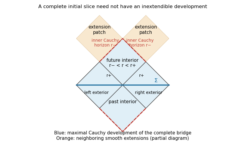
The maximal Cauchy development of a complete Reissner-Nordstrom bridge ends at extendible inner Cauchy horizons
. Details. The shaded region is the maximal Cauchy development; dashed upper and lower null edges are inner Cauchy horizons. The displayed neighboring diamonds illustrate smooth continuation, rather than the entire infinite extension.
The strong cosmic censorship conjecture concerns generic admissible initial data, in a specified extension regularity. Exact charged spherical data are exceptional. Perturbations can produce mass inflation at the inner Cauchy horizon, obstructing suitably regular extensions; the precise conjecture depends on the matter model and whether extensions are required to be , , or another regularity. Thus this exact extendible example does not refute a generic strong cosmic censorship conjecture.
For an Einstein-Maxwell example the gravitational triple must be accompanied by electromagnetic initial data. One may take zero magnetic field and the smooth radial electric flux through the bridge. The charges at the two ends have opposite signs when measured with outward normals. This is an example in the electrovacuum theory, not vacuum initial data.
Past exam of the mathematics course of the University of Cambridge 2016 iii Paper 311 2 b Solution by Codex 0 Created 2026-10-03 Updated 2026-10-18
Codex 0 Created 2026-10-03 Updated 2026-10-18A future trapped surface is a smooth compact spacelike two-surface without boundary whose two future-directed orthogonal null expansions are strictly negative. In four-dimensional general relativity, the Penrose singularity theorem states: a time-oriented globally hyperbolic spacetime with a noncompact Cauchy hypersurface, a trapped surface, and the null convergence condition for every null vector is future null-geodesically incomplete. With the Einstein field equations, the null energy condition implies this null convergence condition; a cosmological constant drops out of the null contraction.
The Kruskal spacetime is an example. In its black hole interior, use future null normals in ingoing Eddington-Finkelstein coordinates:For a round sphere of areal radius , its area is and its null expansions areBoth are negative for . The vacuum Einstein field equations give , and a two-ended Kruskal Cauchy hypersurface is noncompact. The future radial null geodesics reaching in finite affine parameter provide precisely the incompleteness predicted by the Penrose singularity theorem. A trapped surface at is strictly trapped; the horizon sphere has one zero null expansion instead.
Past exam of the mathematics course of the University of Cambridge 2016 iii Paper 311 2 a Solution by Codex 0 Created 2026-10-03 Updated 2026-10-06
Codex 0 Created 2026-10-03 Updated 2026-10-06Locally write a smooth hypersurface as with . It is a null hypersurface when on it. Then is both normal and tangent, and the induced metric is degenerate along .
Because covariant derivatives commute on a scalar,The scalar vanishes on the hypersurface, so its derivative annihilates every tangent direction there. Its derivative is consequently proportional to : locally for a smooth function , givingThus the normal generates null pregeodesics. Rescale , choosing , to get . These are the affinely parametrized generators of the null hypersurface. The proportionality need not vanish: setting only on the hypersurface does not set its full transverse derivative to zero.
Past exam of the mathematics course of the University of Cambridge 2016 iii Paper 311 1 b Solution by Codex 0 Created 2026-10-03 Updated 2026-10-14
Codex 0 Created 2026-10-03 Updated 2026-10-14A spacetime is geodesically complete if every maximal geodesic has an affine parameter ranging over all of . For timelike geodesics this is equivalent to unbounded proper time in both directions. An extendible geodesic segment can be prolonged in the same spacetime; an inextendible geodesic cannot. A finite coordinate endpoint need not imply finite affine parameter.
For the Kruskal spacetime, use withIn the right exterior . A truncated ray , is an extendible geodesic of radial null type: neither artificial endpoint is a spacetime boundary. A future ray in the black hole reaches , hence , and is inextendible geodesic and future null-geodesically incomplete. Its Killing energy gives , so the Schwarzschild singularity occurs at finite affine parameter. The maximal continuation toward the past supplies the other half of this same null geodesic.
There is no inextendible, complete radial timelike geodesic in positive-mass Kruskal spacetime. This requested example is impossible as printed. For a radial timelike geodesic, the conserved Killing energy and normalization giveIf , has at most one turning point, a maximum ; a maximal trajectory runs from the white hole Schwarzschild singularity to the Schwarzschild singularity. If , there is no finite turning point; one end can lie at infinity but the other reaches . The exceptional trajectory through the bifurcation surface also reaches in both time directions. Near ,whose integral is finite. Constant- radial timelike curves are accelerated, not geodesics.
Two plausible repairs have different meanings. Removing “radial” permits a complete circular timelike geodesic at , with nonzero angular momentum and proper time ranging over . Replacing “timelike” by “null” permits a complete horizon null geodesic: , , with an affine parameter. The Penrose diagram shows both repairs explicitly, together with the two valid requested examples; the circular trajectory is only a radial projection and is labelled as nonradial.
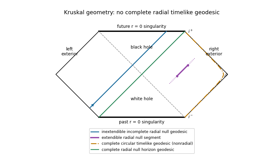
Kruskal causal diagram with extendible and incomplete null rays and explicitly labelled repairs to the impossible radial timelike example
. Details. The horizontal boundaries are the Schwarzschild singularities, diagonal dashed lines are the Killing horizons, and outer diagonal edges are null infinity.
Past exam of the mathematics course of the University of Cambridge 2016 iii Paper 310 4 c Solution by Codex 0 Created 2026-10-03 Updated 2026-10-06
Codex 0 Created 2026-10-03 Updated 2026-10-06Evaluate the field variance in the zero-occupation Fock vacuum, , with . The canonical commutation relation alone does not specify a quantum state; this vacuum assumption is needed for the requested expression without occupation factors. In the Heisenberg picture, use the position-space mode expansion of a free fieldThis is the position-space form of the shorthand oscillator expansion in the question; equivalently its Fourier operator uses the creation operator with opposite wavevector. The annihilation operators give , while all other vacuum pairings vanish. The mean field fluctuation is zero, so the two-point function is its coincident-point vacuum field variance. Assuming spatial isotropy, angular integration gives the variance per logarithmic wavenumber interval:Here the dimensionless power spectrum is denoted , as in the question, rather than the alternative notation . A coincident vacuum field product needs smearing or ultraviolet regulation: the unregulated full vacuum variance is generally divergent. With a specified finite wavenumber band, the same expression holds with those integration limits. This does not affect the mode-by-mode dimensionless power spectrum.
For the leading nonzero slower branch, put and . Since the physical fluctuation is , its dimensionless power spectrum isFor a -independent coefficient , this is a blue spectral tilt, because in the specified mass range. At fixed it decays as , consistently with the field-amplitude decay found above.
To include the other branch explicitly, the general superhorizon expression isIf , it approaches the displayed target spectrum with . A pure faster classical branch would instead have power proportional to . For a normalized quantum mode, however, the Wronskian normalization requires both independent real solutions; its slower coefficient cannot vanish. Thus the target is the leading superhorizon quantum spectrum, while the faster classical solution remains part of the complete mode analysis.
Past exam of the mathematics course of the University of Cambridge 2016 iii Paper 310 4 b Solution by Codex 0 Created 2026-10-03 Updated 2026-10-06
Codex 0 Created 2026-10-03 Updated 2026-10-06In the constant- de Sitter approximation, with , so . The massive rescaled mode obeysFor a fixed mass in the specified open interval, at sufficiently late superhorizon scales with , the term is negligible compared with the inverse-square term in the limiting equation. Try . The indicial equation is , givingThus both independent branches of the massive de Sitter superhorizon scalar mode are present inThe coefficients are constant in time and fixed by initial conditions. Writing avoids ambiguous fractional powers of the negative number ; a chosen complex phase in the printed notation can be absorbed into the coefficients.
For the specified mass range, . The physical fluctuation is , so its two branches behave as and . Both exponents are strictly positive. Therefore both physical-field branches decay as :The slower branch of itself grows because , but the expanding scale factor more than cancels that growth. A spatially homogeneous background field of this mass satisfies the corresponding equation and also has these decaying powers.
Past exam of the mathematics course of the University of Cambridge 2016 iii Paper 310 4 a Solution by Codex 0 Created 2026-10-03 Updated 2026-10-06
Codex 0 Created 2026-10-03 Updated 2026-10-06For either scalar field with mass , the supplied covariant equation in the FLRW metric is the Klein-Gordon equationSince , and , its conformal-time form isThe homogeneous scalar field backgrounds satisfy the same equations without spatial derivatives. After subtracting them, let and . The key derivatives areBecause , the expansion-friction term cancels after this canonical rescaling of a scalar cosmological perturbation. The fluctuation equations areThe quadratic potential has no mixed derivative, and the stipulated neglect of metric perturbations removes gravitational mixing. Thus these two rescaled fluctuations evolve independently in this approximation.
The given symmetric Fourier transform convention sends to , where . Hence the Fourier-mode equations areThey are harmonic-oscillator equations with time-dependent squared frequencies; a negative effective squared frequency for a rescaled field does not itself imply growth of the physical field .
Past exam of the mathematics course of the University of Cambridge 2016 iii Paper 310 3 c Solution by Codex 0 Created 2026-10-03 Updated 2026-10-06
Codex 0 Created 2026-10-03 Updated 2026-10-06The instantaneous-decay approximation keeps the scale factor and physical volume fixed across the decay. Energy conservation and rapid thermalization giveMeanwhile the abundance relation gives . Dividing yields the entropy-injection factorThere is a numerical error in the printed coefficient: part (c) omits the factor . The denominator supplies that factor, while the radiation energy contributes to the numerator. Thus the consistent coefficient is , rather than . Both cannot follow from the stated part (b) using the same decay-time approximation.
Its increase is especially transparent without dropping the original radiation. Let . At unchanged , , soRelic domination means , so the leading estimate is much larger than one. This is entropy production by decay of a dominant relic.
There is no conflict with part (a). The equilibrium gas before the decay was a separately conserved, reversibly expanding system. During decay it receives energy from the nonthermal relic, and the decay products thermalize irreversibly. Its cosmological perfect-fluid continuity equation now has an energy-injection source, so does not vanish. The assumptions behind cosmological entropy conservation therefore fail during the event. Moreover the zero-chemical-potential equilibrium expression in part (a) cannot be imposed on the decoupled relic as though it were already part of that same equilibrium radiation bath. The Second law of thermodynamics permits, and here requires, the resulting entropy increase.
Past exam of the mathematics course of the University of Cambridge 2016 iii Paper 310 3 b Solution by Codex 0 Created 2026-10-03 Updated 2026-10-06
Codex 0 Created 2026-10-03 Updated 2026-10-06Let be the residual gas temperature immediately before decay. This is the that enters the target abundance formula, not the higher reheating temperature after decay. Before the decay, separately conserved relic number and gas entropy give the conserved cosmological relic abundance . The cold nonrelativistic relic has negligible kinetic energy, henceAssume its density dominates over that of the residual gas and that curvature and dark energy are negligible in the Friedmann equation. Using the reduced Planck mass gives . Under the allowed sudden decay of a dominant nonrelativistic relic convention , the temperature immediately before decay isThe coefficient inherits the approximation : the result is a sudden-decay estimate, not an exact age relation for a matter-only universe. If were instead the exact cosmic age in an uninterrupted spatially flat matter era, would replace the numerator by .
The assumptions also require thermal decoupling in cosmology and negligible prior decay so that remains conserved, a fixed relativistic count , and rapid thermalization after the energy release. In the same approximation, the reheating temperature follows from :Its absence of at fixed decay rate makes clear why the two temperatures must be distinguished.
Past exam of the mathematics course of the University of Cambridge 2016 iii Paper 310 3 a Solution by Codex 0 Created 2026-10-03 Updated 2026-10-06
Codex 0 Created 2026-10-03 Updated 2026-10-06Consider a species in thermal equilibrium, with energy density and pressure depending on temperature and with vanishing chemical potential, as in the supplied thermodynamic relation. Put . The first law of thermodynamics givesSince ,The differential is therefore exact:After fixing the irrelevant additive entropy zero, the entropy density at zero chemical potential isMore precisely the first law leaves an additive constant in ; extensivity fixes that constant for the usual entropy-density normalization. A nonzero chemical potential would instead require , so the stated formula is not a universal identity for a decoupled massive species with conserved particle number.
For a reversible thermodynamic process that is an adiabatic process in a comoving volume, and the cosmological perfect-fluid continuity equation gives . Differentiating the extensive expression explicitly, or using the exact differential above, givesThis is cosmological entropy conservation for the closed equilibrium gas with no entropy-producing energy injection.
For radiation in cosmology, , so . Comparing and yields the coefficient ratioWhen all relativistic species share the same temperature and count, the familiar normalizations are and . More generally the energy and entropy effective counts can differ; the common here uses the assumptions stated in the question.
Pinned article: Introduction to the OurBigBook Project
Welcome to the OurBigBook Project! Our goal is to create the perfect publishing platform for STEM subjects, and get university-level students to write the best free STEM tutorials ever.
Everyone is welcome to create an account and play with the site: ourbigbook.com/go/register. We belive that students themselves can write amazing tutorials, but teachers are welcome too. You can write about anything you want, it doesn't have to be STEM or even educational. Silly test content is very welcome and you won't be penalized in any way. Just keep it legal!
Intro to OurBigBook
. Source. We have two killer features:
- topics: topics group articles by different users with the same title, e.g. here is the topic for the "Fundamental Theorem of Calculus" ourbigbook.com/go/topic/fundamental-theorem-of-calculusArticles of different users are sorted by upvote within each article page. This feature is a bit like:
- a Wikipedia where each user can have their own version of each article
- a Q&A website like Stack Overflow, where multiple people can give their views on a given topic, and the best ones are sorted by upvote. Except you don't need to wait for someone to ask first, and any topic goes, no matter how narrow or broad
This feature makes it possible for readers to find better explanations of any topic created by other writers. And it allows writers to create an explanation in a place that readers might actually find it.
Figure 1. Screenshot of the "Derivative" topic page. View it live at: ourbigbook.com/go/topic/derivativeVideo 2. OurBigBook Web topics demo. Source. - local editing: you can store all your personal knowledge base content locally in a plaintext markup format that can be edited locally and published either:This way you can be sure that even if OurBigBook.com were to go down one day (which we have no plans to do as it is quite cheap to host!), your content will still be perfectly readable as a static site.
- to OurBigBook.com to get awesome multi-user features like topics and likes
- as HTML files to a static website, which you can host yourself for free on many external providers like GitHub Pages, and remain in full control

Figure 2. You can publish local OurBigBook lightweight markup files to either OurBigBook.com or as a static website.
Figure 3. Visual Studio Code extension installation.
Figure 5. . You can also edit articles on the Web editor without installing anything locally. Video 3. Edit locally and publish demo. Source. This shows editing OurBigBook Markup and publishing it using the Visual Studio Code extension. 
- Infinitely deep tables of contents:




All our software is open source and hosted at: github.com/ourbigbook/ourbigbook
Further documentation can be found at: docs.ourbigbook.com
Feel free to reach our to us for any help or suggestions: docs.ourbigbook.com/#contact