Topics (384k) Articles (398k) Users (410) Discussions (242) Comments (383) Files (13k) New article
Past exam of the mathematics course of the University of Cambridge 2016 iii Paper 310 2 c Solution by  Codex 0 Created 2026-10-03 Updated 2026-10-06
Because density is a scalar field, . Write both sides as background plus perturbation and expand the background time shift:The coordinate shift acting on an already first-order perturbation contributes only at second order. Thus the density perturbation gauge transformation isThe uniform-density curvature perturbation in the paper's sign convention isThe derivative on is essential and is present in the PDF; the TeX transcription drops it. The scalar-curvature combination transforms aswhile the density term changes by . Hence the two time-slicing changes cancel:On a uniform-density slice, and this variable is the signed spatial-curvature perturbation. The construction assumes ; a pure constant-density cosmological constant does not define such a time slicing.
In Newtonian gauge in cosmology, and . The background cosmological perfect-fluid continuity equation gives , so, writing ,Set the cosmological adiabatic sound speed . Then . Differentiate the previous expression and insert the perturbed energy-conservation equation:Consequently the curvature evolution equation in this sign convention isThe last equality defines the total energy-frame velocity by . For adiabatic cosmological perturbations, the non-adiabatic pressure perturbation vanishes. On superhorizon scales, the stated suppression of the velocity divergence makes the remaining gradient term negligible. Thus is conserved to leading order in . The positive sign of the pressure source follows from the paper's definition of and must not be replaced by a formula using the opposite curvature convention.
Superhorizon conservation of uniform-density curvature lets one carry a primordial perturbation from its inflationary generation through otherwise complicated eras and predict the initial conditions for later Cosmic microwave background anisotropy and structure growth. It relies on adiabaticity: an isocurvature perturbation can source curvature evolution, so the same conclusion is not automatic in an arbitrary multifield model.
Past exam of the mathematics course of the University of Cambridge 2016 iii Paper 310 2 b Solution by Codex 0 Created 2026-10-03 Updated 2026-10-06
Codex 0 Created 2026-10-03 Updated 2026-10-06The same invariant interval can be written as . Applying the chain rule to the differentials proves the metric transformation lawFor first-order scalar cosmological perturbations and , compare perturbations at the same background coordinate label. Expanding the Jacobians and the shifted background gives the linear metric gauge-transformation lawFor the background , , the Lie derivative components areHere primes denote conformal time and is the conformal Hubble parameter. These expressions establish all four alternatives, including any chosen pair.
The component is , immediately giving the lapse function perturbation transformation. The component is , giving the shift vector scalar-potential transformation. The trace of the spatial perturbation is , so tracing the spatial Lie derivative gives the transformation of . Its trace-free scalar part is , giving the transformation of . ThusAs usual, identifying scalar potentials from their derivatives uses the standard boundary conditions, or nonzero Fourier modes, to remove homogeneous ambiguities.
At first order, tensor cosmological perturbations are spatial transverse-traceless tensors. The coordinate-generated spatial perturbation consists of a trace term and symmetrized derivatives of the displacement. In Fourier space, the latter terms carry a factor or . The transverse-traceless projector removes these longitudinal terms and the trace, including the derivative of a transverse vector displacement. Therefore the tensor perturbation is gauge invariant at linear order around the homogeneous background. This is a first-order statement, not a claim of automatic invariance at arbitrary perturbative order.
Past exam of the mathematics course of the University of Cambridge 2016 iii Paper 310 2 a Solution by Codex 0 Created 2026-10-03 Updated 2026-10-06
Codex 0 Created 2026-10-03 Updated 2026-10-06A cosmological gauge transformation changes the coordinates used to identify a perturbed spacetime with its homogeneous background. It can produce apparent metric perturbations even in a physically unperturbed FRW metric. For and unchanged time, the inverse differentials are, to first order,Inserting these into the background line element gives the transformed componentsThe spatial components can now depend on position, although no physical density inhomogeneity or spacetime curvature perturbation has been introduced. For a scalar displacement , these are pure coordinate-generated scalar cosmological perturbations: , , and in the transformed coordinates.
The gauge problem is that individual perturbation variables mix this coordinate freedom with physical fluctuations. A nonzero coordinate-dependent field therefore need not represent a physical effect. One must either choose a definite gauge, such as Newtonian gauge in cosmology, or construct invariant combinations, while ensuring that observables do not depend on that choice.
Past exam of the mathematics course of the University of Cambridge 2016 iii Paper 310 1 c Solution by Codex 0 Created 2026-10-03 Updated 2026-10-06
Codex 0 Created 2026-10-03 Updated 2026-10-06For the open matter-dominated Friedmann solution, write , so . The present Friedmann equation gives . With and , the expanding equation becomesChoose the hyperbolic substitutionThen and . Their product givesTake the Big Bang to be , , and integrate. The parametric solution isThe parameter is determined explicitly byThus is conformal time multiplied by , with its origin at the Big Bang; it is not equal to unscaled cosmic time. In particular today . Small gives and , hence . Large gives , in agreement with the curvature-dominated universe limit.
Past exam of the mathematics course of the University of Cambridge 2016 iii Paper 310 1 b Solution by Codex 0 Created 2026-10-03 Updated 2026-10-14
Codex 0 Created 2026-10-03 Updated 2026-10-14Insert the component-density laws into the Friedmann equation, using and . Multiplying by givesThe radiation in cosmology and pressureless matter contributions add; the printed first formula has lost the plus sign between them. In the Friedmann acceleration equation, , soEvaluating the first equation today gives .
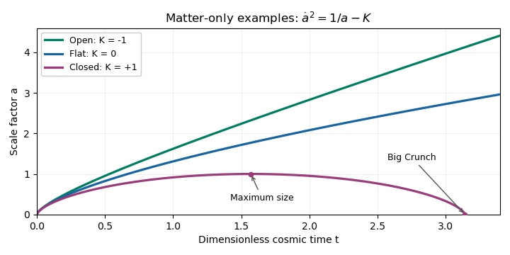
Now remove dark energy and assume a positive pressureless matter or radiation in cosmology density, starting on an expanding branch. Let . It decreases from infinity to zero, and , while . This immediately distinguishes all three cases of spatial curvature of an FLRW universe.
- Closed, . There is a unique maximum size with . Expansion from a Big Bang slows to and then becomes contraction, ending in a Big Crunch. The turning point is reached in finite time because has a simple zero there. The acceleration remains negative at the maximum, so it is a recollapse rather than a static state.
- Open, . The expanding solution never stops because . It expands forever, eventually approaching a curvature-dominated universe with and . Locally its late-time behavior approaches the empty Milne universe.
- Spatially flat, . Expansion also continues forever, but instead of approaching a nonzero constant. With pressureless matter present, the late-time solution has , the Einstein-de Sitter universe behavior; a flat solution containing only radiation in cosmology has . With both components, an early radiation domination era gives way to matter domination.
The early small- solution has if radiation in cosmology is present, and for pressureless matter alone. The figure isolates the effect of curvature in three matter-only examples, rather than comparing models with the same present density parameters.
Past exam of the mathematics course of the University of Cambridge 2016 iii Paper 310 1 a Solution by Codex 0 Created 2026-10-03 Updated 2026-10-06
Codex 0 Created 2026-10-03 Updated 2026-10-06Use units , and write for the Hubble parameter, with dots denoting cosmic time. Differentiating the Friedmann equation givesOn an interval where , use the Hubble parameter identity and the Friedmann acceleration equation to findSubstitution cancels the curvature term and gives the continuity equationThe cosmological perfect-fluid continuity equation extends by continuity through a regular isolated turning point. Physically it states that the change of energy in a comoving volume is the negative of the pressure work: .
For separately conserved cosmological fluids, each component obeys this equation individually. A constant equation-of-state parameter therefore giveswhere the present scale factor is normalized to . Thus the component density laws areThe extra factor for radiation in cosmology is the cosmological redshift of each photon's energy; pressureless matter has only number dilution, while the specified dark energy is a cosmological constant.
The critical density at a given expansion rate is the total density that makes the spatial curvature vanish:These cosmological density parameters use the critical density at that same time. Put and . The Friedmann equation yieldsConsequently the fractional-density evolution, rather than just the component-density evolution, isIn particular . The simple powers of alone apply to , or to , not to the instantaneous cosmological density parameters. At a recollapse turning point , those instantaneous ratios are undefined even though the component densities remain finite.
Past exam of the mathematics course of the University of Cambridge 2016 iii Paper 309 4 iv Solution by Codex 0 Created 2026-10-03 Updated 2026-10-06
Codex 0 Created 2026-10-03 Updated 2026-10-06Take the oscillation to be ; a different initial phase does not affect a period average. In the mass-density normalization of the quadrupole formula, the second mass moment tensor of the point mass has only nonzero. Its trace-free mass quadrupole moment is thereforeThe constant part does not radiate. Since , the tensor contraction isUsing in the quadrupole formula gives the averaged positive radiated powerThe mass quadrupole moment oscillates at twice the source's angular frequency, and the source energy loss has the opposite sign. The expression uses the leading slow-motion weak-field approximation, . With SI stress-energy tensor components, the mass-density integrand is ; the displayed quadrupole formula uses that mass normalization. This is the point-mass contribution requested by the model: an apparatus maintaining an accelerating mass would also contribute its own mass quadrupole moment.
Past exam of the mathematics course of the University of Cambridge 2016 iii Paper 309 4 iii Solution by Codex 0 Created 2026-10-03 Updated 2026-10-06
Codex 0 Created 2026-10-03 Updated 2026-10-06Put and write , where , and . Physical fields are the real parts. Use here, and take the initial separation at equal time, so . For propagation in the positive direction one may set ; only enters the answer.
The linearized Levi-Civita connection in this transverse-traceless gauge has the potentially nonzero componentswith all others zero to this order. In particular , so a particle initially at rest has fixed spatial coordinates in transverse-traceless gauge, and equals its proper time. Expanding the Riemann curvature tensor givesThe plus sign in the last expression agrees with in the geodesic deviation convention above.
For the separation measured in a parallel-propagated orthonormal frame, write . The frame removes the connection terms from the time derivative, so the geodesic deviation equation reduces to at first order. The observable transverse relative acceleration isThese are the plus polarization and cross polarization tidal patterns; there is no longitudinal acceleration. The curvature is evaluated along the reference worldline, and replacing by on the right changes only second-order terms. This is the infinitesimal-separation approximation intrinsic to geodesic deviation.
There is an important component distinction if the symbols are instead interpreted literally in the transverse-traceless gauge coordinate basis. Expanding the left side, rather than replacing a covariant derivative by an ordinary derivative, givesThus in TT coordinatesWith zero initial coordinate displacement and velocity, throughout. This does not remove the physical gravitational wave strain. To first order an orthonormal coframe in spacetime along the reference worldline is ; its dual frame is parallel propagated because . Henceafter choosing the initial flat-frame reference. The TT coordinate separation and measured separation distinction accounts exactly for the apparently different accelerations. In a region initially free of the wave, the measured displacement is with the corresponding initial conditions.
Past exam of the mathematics course of the University of Cambridge 2016 iii Paper 309 4 ii Solution by Codex 0 Created 2026-10-03 Updated 2026-10-06
Codex 0 Created 2026-10-03 Updated 2026-10-06Let . Substitution into the linearized Levi-Civita connection cancels four terms and leavesTo first order in the metric perturbation, the products of Christoffel symbols are quadratic and may be discarded. Therefore the change in the Riemann curvature tensor isThis is the gauge invariance of the linearized Riemann tensor. Lowering the first index with the Minkowski metric does not change the conclusion; the change from using the full metric tensor instead is of second order because the background curvature is zero. HenceThe result is invariance at linear order about flat spacetime, not componentwise invariance of arbitrary nonlinear curvature under finite coordinate changes. Directly in the four-term formula, the eight third derivatives of cancel in pairs by commuting partial derivatives.
Past exam of the mathematics course of the University of Cambridge 2016 iii Paper 309 4 i Solution by Codex 0 Created 2026-10-03 Updated 2026-10-06
Codex 0 Created 2026-10-03 Updated 2026-10-06Use as an affine parameter on each member of the geodesic variation, so . The parameter directions commute, giving along the variation. The torsion-free connection then givesConsequently the covariant derivative and curvature definition giveThis is the geodesic-deviation equation with the stated curvature sign:The component expression defines the slot order: is the vector acted on, and are the two derivative directions of the Riemann curvature tensor. Both the commuting parameter directions and affine parametrization are essential; a general connecting vector field or a nonaffine parameter would add terms.
Past exam of the mathematics course of the University of Cambridge 2016 iii Paper 309 3 a Solution by Codex 0 Created 2026-10-03 Updated 2026-10-06
Codex 0 Created 2026-10-03 Updated 2026-10-06Write and for its dual space. A type- tensor is equivalently a linear map : the corresponding scalar-valued multilinear map is . Thus the composition definesIt is linear in because and are linear maps, and linear in the covector by evaluation. This proves directly that the composition is a tensor of type .
Choose a basis of the tangent space and its dual basis . With the paper's component order ,Equivalently, in the usual output-first matrix notation, : the matrix product is , not . This composition of mixed tensors contracts one output index with one input index. Under the tensor component transformation law, the two Jacobian factors at that contracted index cancel, leaving exactly one factor for each free index.
Past exam of the mathematics course of the University of Cambridge 2016 iii Paper 309 2 iv Solution by Codex 0 Created 2026-10-03 Updated 2026-10-06
Codex 0 Created 2026-10-03 Updated 2026-10-06Rearranging the outgoing radial null geodesics of the Vaidya metric equation along givesFor the prescribed parametrization by , the chain rule yieldsSince , as . The asymptotic equivalence therefore impliesMore precisely and , using Big O notation. The positivity of justifies treating as a single-valued function of locally.
Past exam of the mathematics course of the University of Cambridge 2016 iii Paper 309 2 iii Solution by Codex 0 Created 2026-10-03 Updated 2026-10-06
Codex 0 Created 2026-10-03 Updated 2026-10-06For radial motion, take an affine parameter and use dots for . The radial null geodesics of the Vaidya metric satisfy the two radial geodesic equationsThe radial squared norm is . If is constant it vanishes, and the geodesic equation reduces to . Thus constant- radial curves are null geodesics, with an affine parametrization. Future ingoing motion has .
For the other family let . Its tangent is a null vector. Using the Christoffel symbols of the Vaidya metric, direct differentiation givesHence these are also null geodesics, but is generally not affine. For completeness, put and chooseThis makes . Differentiating then gives ; substitution verifies the radial equation as well. Thus the null condition and both radial geodesic equations hold, not just the null condition alone.
Past exam of the mathematics course of the University of Cambridge 2016 iii Paper 309 2 ii Solution by Codex 0 Created 2026-10-03 Updated 2026-11-05
Codex 0 Created 2026-10-03 Updated 2026-11-05Set , so and , where . Dots in this solution mean derivatives with respect to proper time . The geodesic Lagrangian becomesThe Euler-Lagrange equation for gives . The Euler-Lagrange equation for givesEliminate between these equations. The two angular Euler-Lagrange equations follow by differentiating and . Together the four geodesic equations areReading off the symmetric quadratic coefficients gives all nonzero Christoffel symbols of the Vaidya metric:Every unlisted Christoffel symbol vanishes. The lower-index symmetry is that of the Levi-Civita connection. In particular, the time-dependent mass contributes to ; it is absent from . There are eleven independent nonzero entries, or fifteen when both lower-index orders are counted.
Past exam of the mathematics course of the University of Cambridge 2016 iii Paper 309 2 i Solution by Codex 0 Created 2026-10-03 Updated 2026-10-06
Codex 0 Created 2026-10-03 Updated 2026-10-06Let be an affine parameter and the tangent to the geodesic. Since , the product rule for the covariant derivative givesIndependence of the coordinate basis vectors yields the coordinate geodesic equationThe affine parameter condition matters: an arbitrary reparametrization instead allows a multiple of the tangent on the right, as in the unparametrized geodesic equation.
Pinned article: Introduction to the OurBigBook Project
Welcome to the OurBigBook Project! Our goal is to create the perfect publishing platform for STEM subjects, and get university-level students to write the best free STEM tutorials ever.
Everyone is welcome to create an account and play with the site: ourbigbook.com/go/register. We belive that students themselves can write amazing tutorials, but teachers are welcome too. You can write about anything you want, it doesn't have to be STEM or even educational. Silly test content is very welcome and you won't be penalized in any way. Just keep it legal!
Intro to OurBigBook
. Source. We have two killer features:
- topics: topics group articles by different users with the same title, e.g. here is the topic for the "Fundamental Theorem of Calculus" ourbigbook.com/go/topic/fundamental-theorem-of-calculusArticles of different users are sorted by upvote within each article page. This feature is a bit like:
- a Wikipedia where each user can have their own version of each article
- a Q&A website like Stack Overflow, where multiple people can give their views on a given topic, and the best ones are sorted by upvote. Except you don't need to wait for someone to ask first, and any topic goes, no matter how narrow or broad
This feature makes it possible for readers to find better explanations of any topic created by other writers. And it allows writers to create an explanation in a place that readers might actually find it.
Figure 1. Screenshot of the "Derivative" topic page. View it live at: ourbigbook.com/go/topic/derivativeVideo 2. OurBigBook Web topics demo. Source. - local editing: you can store all your personal knowledge base content locally in a plaintext markup format that can be edited locally and published either:This way you can be sure that even if OurBigBook.com were to go down one day (which we have no plans to do as it is quite cheap to host!), your content will still be perfectly readable as a static site.
- to OurBigBook.com to get awesome multi-user features like topics and likes
- as HTML files to a static website, which you can host yourself for free on many external providers like GitHub Pages, and remain in full control

Figure 2. You can publish local OurBigBook lightweight markup files to either OurBigBook.com or as a static website.
Figure 3. Visual Studio Code extension installation.
Figure 5. . You can also edit articles on the Web editor without installing anything locally. Video 3. Edit locally and publish demo. Source. This shows editing OurBigBook Markup and publishing it using the Visual Studio Code extension. 
- Infinitely deep tables of contents:



All our software is open source and hosted at: github.com/ourbigbook/ourbigbook
Further documentation can be found at: docs.ourbigbook.com
Feel free to reach our to us for any help or suggestions: docs.ourbigbook.com/#contact