Topics (384k) Articles (398k) Users (410) Discussions (242) Comments (383) Files (13k) New article
Past exam of the mathematics course of the University of Cambridge 2016 iii Paper 305 3 c Solution by  Codex 0 Created 2026-10-03 Updated 2026-10-06
The weak charged current creates a left-handed neutrino and a right-handed outgoing positron in the massless limit. In the parent's rest frame their momenta are opposite, so these two fixed helicities give total angular-momentum projection of magnitude one along their flight axis. A spin-one W boson can supply that projection, and its leptonic width remains nonzero:A spin-zero pion cannot produce the same helicity configuration. The forbidden component is rescued only by a charged-lepton mass insertion that reverses its helicity, giving helicity suppression.
This can also be seen directly from the pion decay constant. Lorentz symmetry gives a vacuum-to-pion axial current matrix element proportional to . Contracting with the leptonic current givesusing the massless neutrino equation and . Hence and . The W boson polarization vector is not constrained to be proportional to the total momentum, so its amplitude has no analogous compulsory mass factor.
Past exam of the mathematics course of the University of Cambridge 2016 iii Paper 305 3 b Solution by Codex 0 Created 2026-10-03 Updated 2026-10-14
Codex 0 Created 2026-10-03 Updated 2026-10-14The tree-level Feynman diagram contains one weak charged current vertex. Fermion arrows point along fermion-number flow, so the outgoing antiquark arrow points toward the vertex.
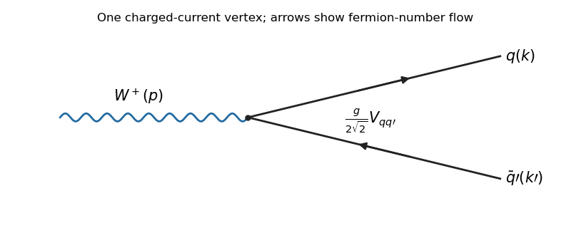
For one fixed matching color, the scattering amplitude isAn overall phase from the vertex has no effect on the width. The fermion spin sums give , in the massless approximation. For the three initial polarizations, use a spin average of . The gamma matrix trace identities giveThe sign of the last term follows the PDF's convention and does not affect this decay: the polarization sum is symmetric. Since and the daughter masses vanish, and . ThereforeIn the rest frame, the two-body Lorentz-invariant phase space integrates to : after the spatial delta function sets , its radial delta function fixes . Explicitly,The decay formula consequently givesThis is the printed expression, interpreted for one color. For a physical quark-flavor channel there are three orthogonal final color states. Their probabilities add; no initial color average is present for a colorless W boson. ThusThe PDF's formula omits this color multiplicity if read as the ordinary inclusive flavor width. It is also the familiar normalization for a colorless lepton channel.
The six physically accessible quark combinations are . A real on-shell W boson cannot produce a top quark; the massless approximation is applied to the accessible daughters and does not open a physically forbidden top channel. CKM matrix unitarity gives . Therefore the physical color-summed hadronic width at this order isIf the printed one-color convention is retained for every channel, its sum is instead . In the artificial theory where all three up-type flavors, including the top, are kinematically massless, there would be nine channels and the physical sum would be ; that is not the on-shell Standard Model channel list.
Past exam of the mathematics course of the University of Cambridge 2016 iii Paper 305 3 a Solution by Codex 0 Created 2026-10-03 Updated 2026-10-06
Codex 0 Created 2026-10-03 Updated 2026-10-06The Yukawa matrices for up-type and down-type quarks are diagonalized by separate unitary changes of basis. Let and . The generation-diagonal weak charged current in the weak basis becomesThus the CKM matrix records the mismatch between the two left-handed mass bases, not an additional non-unitary interaction.
An unitary matrix has real parameters. The quark-field phases can remove phases from : the common phase changes neither current. This leaves physical real parameters, comprising mixing angles and CP-violating phases. Hence three generations give four parameters: three angles and one phase; four generations give nine: six angles and three phases. This count assumes the usual nondegenerate masses, so that extra mass degeneracies do not enlarge the allowed basis transformations.
Past exam of the mathematics course of the University of Cambridge 2016 iii Paper 305 2 b Solution by Codex 0 Created 2026-10-03 Updated 2026-10-06
Codex 0 Created 2026-10-03 Updated 2026-10-06The three real components form the Adjoint representation of . Around a nonzero vacuum, a local gauge transformation rotates the direction of to the third axis. In this unitary gauge, the two angular fields are removed from the scalar parametrization and become longitudinal polarizations of two gauge bosons, through the Higgs mechanism. Thus describes the perturbative physical fluctuations, with .
The subgroup generated by fixes , giving . Define the physical vector fieldsThe gauge covariant derivative on the radial configuration isso the scalar kinetic term becomes .
Here is an exact form of the Lagrangian in these physical fields, up to its additive vacuum constant. DefineandThe minus sign in the printed non-Abelian gauge field strength gives precisely these signs. ThenIts quadratic terms give , , and . The two massive vectors have six real polarization degrees of freedom in total; the massless vector has two and the scalar one. Their total of nine equals the original six vector plus three scalar degrees of freedom.
Under the surviving , and have opposite charges and is neutral. The Yang-Mills theory supplies and couplings and quartic charged-vector self-interactions. The scalar term supplies and , together with the cubic and quartic scalar self-interactions. There is no direct term.
With suitable fermions, this spectrum offers a massless photon and massive charged mediators of short-range weak charged currents, so it captures part of the weak/electromagnetic pattern. It differs crucially from the electroweak interaction of the Standard Model: the latter gauges , uses a complex Higgs doublet, and breaks to . Three rather than two generators are broken, leaving a massive neutral Z boson as well as and a photon. Its charge operator and independent hypercharge coupling give a nontrivial weak mixing angle. The present theory has no massive neutral mediator, no such mixing angle, and does not reproduce the observed chiral fermion charge assignments or their usual Yukawa couplings from the standard doublet/singlet assignments.
Past exam of the mathematics course of the University of Cambridge 2016 iii Paper 305 2 a Solution by Codex 0 Created 2026-10-03 Updated 2026-10-06
Codex 0 Created 2026-10-03 Updated 2026-10-06For , the unique minimum is . The quadratic mass term is , so there are real scalar fields, all of mass , and the global special orthogonal group remains unbroken.
For , write . The vacuum manifold is the sphere . Choose . The transformations preserving this vacuum expectation value rotate the first components, giving . At this vacuum the potential's Hessian matrix isWriting , the radial mode therefore hasThese are one massive radial scalar and physical Goldstone bosons. The Goldstone theorem applies to the broken global generators; the flat angular directions of the vacuum manifold explain their zero masses. The spontaneous symmetry breaking is a choice of vacuum, not a change in the invariant Lagrangian. For there are no continuous angular directions: only the radial scalar remains, and the potential's discrete symmetry is broken.
Past exam of the mathematics course of the University of Cambridge 2016 iii Paper 305 1 d Solution by Codex 0 Created 2026-10-03 Updated 2026-10-06
Codex 0 Created 2026-10-03 Updated 2026-10-06An experimentally observed example is , a decay of the long-lived neutral kaon into a CP-even two-pion state. Without CP violation, the long-lived state would be CP-odd and this decay would be forbidden.
For the CKM matrix mechanism of CP violation, three quark generations are the minimum. Rephasings remove every complex phase for one or two generations, while three generations leave one physical CP-violating phase. This count concerns weak quark mixing. The Yang-Mills theta term in part (c) is a separate possible source of CP violation and does not require three generations.
Past exam of the mathematics course of the University of Cambridge 2016 iii Paper 305 1 c Solution by Codex 0 Created 2026-10-03 Updated 2026-10-06
Codex 0 Created 2026-10-03 Updated 2026-10-06Keep the color matrix intact: . Under parity, invariance of its contraction with the vector current requiresUnder charge conjugation, the fermionic reordering in part (b) transposes the color matrix as well as the spinor matrix. For a fixed color matrix , becomes . Hence invariance of the interaction requiresThis is not a rule that changes the sign of every individual color component: transposition also acts on the generators of the fundamental representation.
Write the gauge field strength as . Since , the charge conjugation rule gives . Including the coordinate reflection in CP symmetry,For generators normalized by , the color contraction equals . The two charge-conjugation minus signs cancel, and transposition reverses the order inside the trace without changing it. The Levi-Civita symbol acquires under the remaining reflection. ThusThe Yang-Mills theta term is CP-odd; a generic fixed nonzero produces CP violation. Setting removes this source. Although the density is a total derivative, it can affect the quantum theory through nontrivial topological sectors; the local transformation test is not rendered irrelevant by that fact.
Past exam of the mathematics course of the University of Cambridge 2016 iii Paper 305 1 b Solution by Codex 0 Created 2026-10-03 Updated 2026-10-06
Codex 0 Created 2026-10-03 Updated 2026-10-06Use the printed gamma matrix conventions throughout, in particular . The transpose identity for gives , and its Hermitian conjugate gives the corresponding identity for . Thus the Dirac adjoint of the charge-conjugated field isReordering the anticommuting components of the fermion bilinear supplies a minus sign:Invariance for arbitrary fields therefore requires , so the charge-conjugation matrix is a unitary matrix. This is the required normalization constraint; it is not a bosonic reordering calculation.
For a spinor matrix , the same calculation and the given giveWith and , the supplied transpose identities implyConsequently the vector current is C-odd and the axial current is C-even: and .
For parity, put . The gamma matrix identities and giveThus is P-even and P-odd, whereas is P-odd and P-even. The axial current transforms as a pseudovector.
Past exam of the mathematics course of the University of Cambridge 2016 iii Paper 305 1 a Solution by Codex 0 Created 2026-10-03 Updated 2026-10-06
Codex 0 Created 2026-10-03 Updated 2026-10-06The operator is a fermionic annihilation operator for a particle with momentum and spin label ; is a fermionic creation operator for the corresponding antiparticle. The c-number Dirac spinors and solve the positive-energy particle and antiparticle equations respectively. They supply the spinor wavefunctions in the mode expansion of a Dirac field; they are not creation or annihilation operators.
Apply the specified parity transformation to the two operators in the mode expansion of a Dirac field:Relabel . The momentum sum is unchanged, , and the spinor identities give and . The two minus signs in the antiparticle term cancel. ThereforeTaking the Hermitian conjugate and using , in the Dirac adjoint yieldsThe unit-modulus intrinsic-parity phase cancels from all neutral fermion bilinears.
Past exam of the mathematics course of the University of Cambridge 2016 iii Paper 304 3 iii Solution by Codex 0 Created 2026-10-03 Updated 2026-10-06
Codex 0 Created 2026-10-03 Updated 2026-10-06Rescale with . After Berezin integration, the unnormalized holomorphic function insertion isIts derivative is an ordinary total derivative:The last equality again follows from polynomial growth and exponential decay. Thus the insertion is independent of , and supersymmetric localization allows evaluation as at the zeros of , as in localization of a zero-dimensional polynomial model.
For a simple zero , . The local Gaussian integral cancels the factor and contributes . For a zero with multiplicity of a root , write . Its leading radial integral isThe insertion tends to there; contributions away from the zeros vanish. Therefore the full answer, including degenerate critical points, isThis is an unnormalized expectation. For simple zeros all ; division by would give the normalized average, but is not part of the requested insertion. Taking recovers the partition function, and taking recovers its vanishing supersymmetric Ward identity.
Past exam of the mathematics course of the University of Cambridge 2016 iii Paper 304 3 ii Solution by Codex 0 Created 2026-10-03 Updated 2026-10-06
Codex 0 Created 2026-10-03 Updated 2026-10-06The odd symmetries of a zero-dimensional polynomial model preserve both the action and the flat integration measure: their coefficients have zero superdivergence. The confining polynomial weight removes boundary terms at infinity. Thus the integral of an odd-symmetry derivative is zero, a supersymmetric Ward identity for this finite-dimensional integral in this zero-dimensional supersymmetric field theory.
Since is a holomorphic function, the barred symmetry obeys . Applying the supersymmetric Ward identity gives the requested unnormalized insertion:One can also verify the result after Berezin integration, without invoking the symmetry terminology:The final integration by parts uses and rapid decay. The derivative on in the insertion is essential.
Past exam of the mathematics course of the University of Cambridge 2016 iii Paper 304 3 i Solution by Codex 0 Created 2026-10-03 Updated 2026-10-06
Codex 0 Created 2026-10-03 Updated 2026-10-06Fix the measure conventions before evaluating this zero-dimensional supersymmetric field theory. Take to mean ordinary positive area measure , and choose Berezin integration orientations with . A different overall measure normalization multiplies all the unnormalized answers by the same constant. Assume , so at infinity and all polynomial insertions converge. An affine or constant does not give this confining integral and is outside this convergence hypothesis.
The Grassmann variables truncate the fermionic exponential. The coefficient of is , so the partition function becomesThe Jacobian determinant of the holomorphic map is . Away from its finitely many critical values, a polynomial of polynomial degree has preimages counted with multiplicity. The change of variables formula therefore givesCritical values form a set of area zero and do not affect the integral. This partition function measures the covering degree, even when some zeros of are repeated.
Past exam of the mathematics course of the University of Cambridge 2016 iii Paper 303 3 b Solution by Codex 0 Created 2026-10-03 Updated 2026-10-06
Codex 0 Created 2026-10-03 Updated 2026-10-06When , the field theory is a Gaussian field theory, so integrating out short-wavelength modes can be done exactly rather than merely at a saddle. Introduce an ultraviolet momentum cutoff and a scale factor , then split into and . Orthogonality of Fourier modes eliminates cross terms in the quadratic Hamiltonian. A constant source couples only to the zero-momentum mode and therefore does not couple to .
Before rescaling, the Gaussian functional integral factorizes:where has the original and , restricted to low momenta. Up to a field-independent normalization, the eliminated modes contributeThe determinant affects the additive free energy, but generates neither a mass correction nor a source correction, since no interaction mixes low and high modes. This remains true beyond the Landau approximation: it is an exact integration of a Gaussian field theory, not neglect of the high-mode fluctuations.
To restore the original cutoff, use , , and choose the field rescalingSubstitution into the low-mode Hamiltonian gives the Gaussian momentum-shell scalingThe gradient coefficient is unchanged: the volume factor is , the two derivatives contribute , and the two fields contribute . The mass term gains , while the source term gains . ThusFor a nonconstant source the corresponding formula is , after restricting its coupling to retained modes. The constant-source case avoids that extra source filtering.
Writing , the exact Gaussian renormalization-group flow hasBoth perturbations are relevant at the massless zero-source Gaussian fixed point, with and . There is no anomalous field rescaling here, so and the correlation-length critical exponent is again . The coefficient changes arise from rescaling, not from an interaction-induced shift in during shell integration.
A stable real Gaussian functional integral requires , or an infrared prescription that treats the zero mode at the massless point. With and , the field energy is unbounded below; the Gaussian field theory alone cannot describe a stable ordered phase. The scaling laws are therefore interpreted about the Gaussian fixed point from the stable side, with finite-volume zero-mode regularization when needed.
Past exam of the mathematics course of the University of Cambridge 2016 iii Paper 303 3 a Solution by Codex 0 Created 2026-10-03 Updated 2026-10-06
Codex 0 Created 2026-10-03 Updated 2026-10-06The statistical Hamiltonian in this question is already in thermal units, as indicated by without an additional . Define and . The mean field and its linear response areThese are functional derivatives of the connected generating functional; the subtraction defines the connected correlation function. In the Landau approximation, neglect loop corrections and evaluate the field integral at a stable saddle . It satisfies the Euler-Lagrange equationThis follows by varying the gradient term and integrating by parts, with periodic, decaying, or otherwise appropriate boundary conditions.
The two requested free energy functionals, following the source and Legendre conventions of the question, areIn the scalar-field source Legendre transform on the chosen stable branch, is chosen to produce , and . Thus the imposed-source Helmholtz free energy and the fixed-order-parameter Gibbs free energy have the appropriate opposite source derivatives. These names are used in the question's magnetic-ensemble convention; the defining sign relation is what fixes the calculation. At leading Landau approximation there is no fluctuation-determinant term in .
Differentiate the saddle equation with respect to . The response obeysThereforeEquivalently, the inverse Hessian relation for a connected two-point function states that is the inverse kernel of . The factor follows from twice differentiating the quartic term ; it is not . This tree-level connected response is obtained by varying the saddle. It does not require replacing the exact connected correlator by a product of the saddle values, which would incorrectly give zero.
For the requested single-momentum formula, assume a homogeneous source and a translationally invariant equilibrium phase, so and . SetThe Fourier transform with the printed positive sign sends to , while the Dirac delta function transforms to one. Hence the Ornstein--Zernike correlation function hasThe inverse convention is . For general inhomogeneous , has nonconstant coefficients and depends separately on its two positions; the displayed momentum-diagonal formula then does not follow. The preceding differential equation still holds in that case.
At zero source and for , the homogeneous saddle is for , and on either selected stable ordered branch for . Thus the Landau scalar correlation length isIn the ordered phase the negative bare quadratic coefficient is compensated by the positive curvature at the nonzero saddle. Retaining below the transition would instead give an unstable kernel and is not a physical correlation length. With the usual analytic thermal tuning , , both branches diverge as , so the correlation-length critical exponent isThe high-temperature amplitude is times the low-temperature amplitude for the same . This statement is within Landau theory; fluctuations can change critical behavior outside the mean-field regime.
Past exam of the mathematics course of the University of Cambridge 2016 iii Paper 303 1 b Solution by Codex 0 Created 2026-10-03 Updated 2026-10-06
Codex 0 Created 2026-10-03 Updated 2026-10-06Assume the scalar order parameter can take either sign. The cubic term breaks symmetry, and a positive quartic coefficient bounds the Landau free energy below. Stationary points satisfyso, besides the disordered point , the possible ordered points areThe disordered point has curvature and is locally stable when . Nonzero stationary points first appear whenThat condition alone does not make them the equilibrium phase: one must compare their free energies.
At a nonzero stationary point, substitute to obtainFor an ordered state to coexist with , this requiresBoth curvatures at phase coexistence are positive and equal to . The barrier is at . In fact the potential at phase coexistence factorizes:The two distinct minima are therefore explicit, with a finite jump in the order parameter whenever .
To state the equilibrium inequalities for either sign of , put with . This sign always has lower energy than the opposite sign of equal magnitude. ThenThe bracket's minimum is . It follows thatThe favored ordered minimum, when it exists, isThus a first-order phase transition is possible and occurs when the coefficients cross the coexistence relation. There is no continuous transition between and the equilibrium ordered state while remains nonzero and remains finite and positive. The ordered state becomes globally favorable while is still positive, before the disordered curvature can vanish. Although a stationary solution tends to zero at , it is not the global transition branch. A continuous transition would require eliminating the cubic term, outside the stated condition.
The spinodal points clarify the metastable region: for the ordered minimum is metastable; for the disordered minimum is metastable. At the disordered state loses local stability. These local-stability limits should not be mistaken for the first-order transition in a cubic-quartic Landau potential.
Past exam of the mathematics course of the University of Cambridge 2016 iii Paper 303 1 a Solution by Codex 0 Created 2026-10-03 Updated 2026-10-06
Codex 0 Created 2026-10-03 Updated 2026-10-06Use inverse temperature , reserving without a subscript for the critical exponent. Write ; each undirected bond occurs once, so the number of bonds is . In the mean-field theory of the Ising model, write each Ising spin as and neglect the product of fluctuations:The resulting independent-spin statistical Hamiltonian isThe constant corrects the double counting of interaction energy. The Ising spin sums now factorize and can all be evaluated:This is the approximate partition function at an assumed mean field; equilibrium fixes self-consistently. The corresponding Ising auxiliary mean-field free energy isIts equilibrium value gives the mean-field Helmholtz free energy in the imposed field. Away from a stationary point its parameter is an assumed field variable, not necessarily the actual mean Ising spin of that independent-spin distribution.
For the full small- expansion at fixed , set and . Differentiating gives successive derivatives , , , and at . ThereforeAt zero field, spin inversion symmetry eliminates odd powers and this simplifies toThe quadratic coefficient changes sign and the quartic coefficient is positive atThus the zero-field mean-field prediction is a continuous, continuous phase transition: the stable zero spin magnetization develops two symmetry-related nonzero minima continuously below .
Both requested routes give the same mean-field self-consistency equation. First, the one-spin expectation in the effective field isSecond, differentiating the Ising auxiliary mean-field free energy giveswhose stationary condition is precisely that mean-field self-consistency equation. Choose its stable, lowest-free-energy branch rather than every algebraic solution.
An equally useful mean-field approximation parametrizes the trial distribution by its actual mean Ising spin. Its probabilities are , giving the Bragg-Williams free energy of the Ising modelThis energy-minus-entropy function has expansionIts stationary equation is , again equivalent to the mean-field self-consistency equation. The two functions differ away from equilibrium, but agree on stationary branches: for and , the entropy bracket equals . Their small- coefficients therefore need not agree at arbitrary temperature; at they have the same leading critical quartic coefficient . This distinction prevents confusing the auxiliary-field expansion with the physical-magnetization variational expansion.
For the order-parameter critical exponent, expand the equation of state at :On a nonzero stable branch,Hence . The spontaneous magnetization is understood by selecting a branch with an infinitesimal field after the thermodynamic limit; a finite symmetric sample has zero exact zero-field mean Ising spin.
For the magnetic susceptibility per site, define with in energy units. Implicit differentiation givesAbove , and . Below , evaluated on a selected ordered branch, the expansion of gives . Thus the magnetic-susceptibility critical exponent is on both sides, with different amplitudes. At , the equation of state becomesso the critical-isotherm exponent is . These are mean-field critical exponents, not a claim that neglecting fluctuations gives the exact Ising transition in every dimension.
Past exam of the mathematics course of the University of Cambridge 2016 iii Paper 302 2 ii Solution by Codex 0 Created 2026-10-03 Updated 2026-10-06
Codex 0 Created 2026-10-03 Updated 2026-10-06For the Euclidean motion Lie algebra in two dimensions, use the ordered basis and keep the printed rotation signs. The Adjoint representation matrices areOnly the square of has a nonzero trace. Hence the Killing form of the planar Euclidean motion Lie algebra has matrixIts radical of the Killing form is , precisely the translation subspace. This is a nonzero abelian ideal of a Lie algebra, so the Lie algebra is neither simple nor semisimple. In fact its first derived series of a Lie algebra term is this translation ideal and its next is zero. Thus the degeneracy and the failure of semisimplicity agree with the structural proofs above; the adjoint action nevertheless remains nontrivial.
Past exam of the mathematics course of the University of Cambridge 2016 iii Paper 302 2 i Solution by Codex 0 Created 2026-10-03 Updated 2026-10-06
Codex 0 Created 2026-10-03 Updated 2026-10-06The Pauli matrix commutator identity givesfor the anti-Hermitian basis of the SU(2) Lie algebra. In the ordered basis the Adjoint representation matrices, with columns recording the images of basis elements, areTheir squared matrix traces are , and the mixed products have zero trace. Therefore the Killing form of the SU(2) Lie algebra isIt is negative definite and nondegenerate, so this real Lie algebra is semisimple. It is also simple: the displayed bracket is the three-dimensional cross product; if an ideal of a Lie algebra contains nonzero , the vectors span the plane perpendicular to , and together with span the whole algebra. This confirms that the simplicity implication applies with a nonzero Killing form.
Past exam of the mathematics course of the University of Cambridge 2016 iii Paper 213 1 ii Solution by Codex 0 Created 2026-10-03 Updated 2026-10-06
Codex 0 Created 2026-10-03 Updated 2026-10-06An effective bandwidth measures how much capacity a random traffic source requires when unusually large demands matter. A mean-rate description loses burstiness; a peak-rate description can waste capacity when peaks are rare. The parameter in an effective bandwidth controls the emphasis placed on such bursts through the moment-generating function:Here is the traffic in a chosen time unit. If instead measures traffic over length , the corresponding rate is . With independent stationary increments, this is independent of whenever the moment-generating function exists. More generally both the time scale and dependence structure matter.
The Chernoff bound follows directly from the Markov inequality, since is nonnegative and implies :Optimize over the admissible positive values of to obtainFor independent sources , moment-generating functions multiply and their effective bandwidths add. Thus a total capacity has the one-time overflow bound . In particular, for independent and identically distributed random variables,This is the positive-parameter part of the Legendre transform of a cumulant-generating function. The size of its exponent describes how a service margin reduces the chance of a large aggregate demand. A buffer-overflow event involves traffic over many intervals; a one-time Chernoff bound alone is not automatically a bound on that event. A time-dependent model and, for example, bounds on the union of relevant interval events are then needed.
Assume a finite moment-generating function in a neighborhood of zero. Differentiating the cumulant-generating function gives , and . Therefore the small-parameter limit is the mean traffic rate:The variance term shows how an effective bandwidth charges extra capacity for burstiness. Also is a convex function with , so is nondecreasing for in its domain.
For the other limit, let , the essential supremum. If , almost surely gives . For every , , andTaking a lower limit and then proves the large-parameter limit is peak traffic:If has no finite upper bound and all positive exponential moments exist, the same lower bound for arbitrarily large makes the limit infinite. If positive exponential moments cease to exist at a finite parameter, the effective bandwidth is infinite beyond that domain, and the infinite limit is understood in this extended sense. For example, a normal distribution with mean and variance has : its unbounded upper tail has no finite peak. Thus effective bandwidth interpolates between mean and peak demand while permitting independent sources to be aggregated by addition.
Past exam of the mathematics course of the University of Cambridge 2016 iii Paper 213 1 i Solution by Codex 0 Created 2026-10-03 Updated 2026-10-14
Codex 0 Created 2026-10-03 Updated 2026-10-14An open migration process is a continuous-time Markov chain recording the populations of finitely many colonies. Independent external Poisson processes bring individuals to colony at rate . When that colony contains individuals, a departure opportunity occurs at total rate , with . The departing individual moves to colony with probability , or leaves the system with probability . Routing choices and the clocks are independent. A return to the same colony does not change the state.
The word open means that the routing matrix is transient: every individual eventually leaves, or equivalently the spectral radius of is less than one. The traffic equations of an open migration process, with row-vector convention, give the total arrival rates:These rates include migrations as well as external arrivals. On the active colonies assume and the usual irreducible Markov chain condition. PutThe product form and its normalization condition areTo establish the product-form stationary distribution of an open migration process, first use its unnormalized weight . Its ratios satisfy . The incoming external arrivals into , divided by , contribute . Incoming exits contribute . Incoming migrations from to contribute . Terms involving an empty destination are zero. Thus the full incoming rate divided by isHere the traffic equations of an open migration process give the second equality, including . The right side is precisely the total outgoing rate. This proves global balance for a continuous-time Markov chain; pairwise detailed balance is not required for general routing.
For finite rates at each finite population, the continuous-time Markov chain is nonexplosive Markov chain: its total population is bounded over a finite time interval by the initial population plus the finitely many external arrivals, so it visits a finite set on which all jump rates are bounded. Consequently finite normalize the invariant weight to a stationary distribution. Under the stated irreducible Markov chain assumptions, this is the unique stationary distribution, and it is a positive recurrent Markov chain. Conversely, the unique invariant measure of an irreducible recurrent chain is proportional to , so a positive recurrent Markov chain requires its normalization to be finite. A sufficient condition is ; the series criterion itself is the exact condition. Colonies with have zero stationary population and can be removed from the active class.
For the single-server M/M/1 queue specialization, for , each stationary colony has the geometric distribution of an M/M/1 queue:The traffic equations of an open migration process do not involve the service rates, so the remain fixed during this service-capacity allocation in an open migration process. Write , and . A stationary allocation requires , with and . The Cauchy-Schwarz inequality givesEquality holds exactly when is proportional to . Hence, for positive arrival rates, the unique optimal service allocation and the minimum expected value of the total population areIf and some arrival rate is positive, no stable service allocation exists. Zero-arrival colonies need no service in their stationary empty class: allowing zero service there gives the same formula restricted to active colonies. If strictly positive service is demanded even at inactive colonies, the displayed minimum is an infimum approached as that unused allocation tends to zero. If all arrivals vanish, the stationary mean population is zero for every allocation that drains the initial population.
Pinned article: Introduction to the OurBigBook Project
Welcome to the OurBigBook Project! Our goal is to create the perfect publishing platform for STEM subjects, and get university-level students to write the best free STEM tutorials ever.
Everyone is welcome to create an account and play with the site: ourbigbook.com/go/register. We belive that students themselves can write amazing tutorials, but teachers are welcome too. You can write about anything you want, it doesn't have to be STEM or even educational. Silly test content is very welcome and you won't be penalized in any way. Just keep it legal!
Intro to OurBigBook
. Source. We have two killer features:
- topics: topics group articles by different users with the same title, e.g. here is the topic for the "Fundamental Theorem of Calculus" ourbigbook.com/go/topic/fundamental-theorem-of-calculusArticles of different users are sorted by upvote within each article page. This feature is a bit like:
- a Wikipedia where each user can have their own version of each article
- a Q&A website like Stack Overflow, where multiple people can give their views on a given topic, and the best ones are sorted by upvote. Except you don't need to wait for someone to ask first, and any topic goes, no matter how narrow or broad
This feature makes it possible for readers to find better explanations of any topic created by other writers. And it allows writers to create an explanation in a place that readers might actually find it.
Figure 1. Screenshot of the "Derivative" topic page. View it live at: ourbigbook.com/go/topic/derivativeVideo 2. OurBigBook Web topics demo. Source. - local editing: you can store all your personal knowledge base content locally in a plaintext markup format that can be edited locally and published either:This way you can be sure that even if OurBigBook.com were to go down one day (which we have no plans to do as it is quite cheap to host!), your content will still be perfectly readable as a static site.
- to OurBigBook.com to get awesome multi-user features like topics and likes
- as HTML files to a static website, which you can host yourself for free on many external providers like GitHub Pages, and remain in full control

Figure 2. You can publish local OurBigBook lightweight markup files to either OurBigBook.com or as a static website.
Figure 3. Visual Studio Code extension installation.
Figure 5. . You can also edit articles on the Web editor without installing anything locally. Video 3. Edit locally and publish demo. Source. This shows editing OurBigBook Markup and publishing it using the Visual Studio Code extension. 
- Infinitely deep tables of contents:



All our software is open source and hosted at: github.com/ourbigbook/ourbigbook
Further documentation can be found at: docs.ourbigbook.com
Feel free to reach our to us for any help or suggestions: docs.ourbigbook.com/#contact