Topics (384k) Articles (398k) Users (410) Discussions (242) Comments (383) Files (13k) New article
Past exam of the mathematics course of the University of Cambridge 2016 iii Paper 320 4 e Solution by  Codex 0 Created 2026-10-03 Updated 2026-10-06
False. The enclosed-mass formula is a consequence of the spherical shell theorem. In a spherical galaxy, exterior shells exert no radial force and interior mass acts as though concentrated at the centre, giving .
A razor-thin axisymmetric disc instead hasBoth interior and exterior annuli contribute to that derivative. Its geometry is not determined by .
A concrete counterexample compares a central point mass plus an exterior spherical shell with the same point mass plus a thin circular ring of mass and radius . Their enclosed-mass profiles are identical: inside , and outside. The interior gravitational force of an exterior thin ring follows by expanding its angularly averaged relative potential:For , the ring's acceleration is outward, , whereas the spherical shell's acceleration is zero. With large enough to retain circular orbits, the disc-side speed isA narrow smooth annulus gives the same distinction. This proves that enclosed mass does not determine a disc rotation curve, even when the mass profiles of the spherical and disc models agree.
Past exam of the mathematics course of the University of Cambridge 2016 iii Paper 320 4 d Solution by Codex 0 Created 2026-10-03 Updated 2026-10-06
Codex 0 Created 2026-10-03 Updated 2026-10-06False. Adiabatic invariance of an orbital action preserves actions under sufficiently slow regular evolution, not the ratios of their frequencies. With action-angle variables, can change even when does not. A closed bound orbit requires commensurate radial and angular frequencies; rational commensurability is not an adiabatic invariant.
For an explicit counterexample, slowly change the physical potential from Kepler form towith a small, slowly varying positive . The radial epicyclic frequency and circular angular frequency at a nearly circular orbit areInitially their ratio is one. For generic nonzero , is irrational, producing the Kepler-harmonic epicyclic precession. An initially slightly eccentric ellipse with nonzero radial action therefore becomes a precessing nonclosed orbit, while its radial action remains approximately fixed and its angular momentum remains exactly fixed by spherical symmetry.
Past exam of the mathematics course of the University of Cambridge 2016 iii Paper 320 4 c Solution by Codex 0 Created 2026-10-03 Updated 2026-10-06
Codex 0 Created 2026-10-03 Updated 2026-10-06False. The singular isothermal sphere is infinite in extent and mass. The isolated finite-system virial theorem cannot be applied to its global divergent energies without boundary terms.
A direct Spherical Jeans equation counterexample is enough. For isotropic velocities with constant one-dimensional dispersion , its density slope givesThus and the circular and isotropic speed comparison in a singular isothermal sphere isThis is realized by a positive isotropic distribution , which gives a Maxwell-Boltzmann distribution of velocities and . Circular orbits have instead and , so their total mean square speed is . The isotropic model contains eccentric orbits except for a measure-zero subset.
The boundary virial term of a singular isothermal sphere explains the different energy budgets of a finite spherical region. At radius , its radial-pressure surface term is . It is nonzero in the isotropic model and zero in the circular-orbit model. Equality of the density therefore does not enforce equality of the velocity energy through an incorrectly omitted surface term.
Past exam of the mathematics course of the University of Cambridge 2016 iii Paper 320 4 b Solution by Codex 0 Created 2026-10-03 Updated 2026-10-06
Codex 0 Created 2026-10-03 Updated 2026-10-06False as a claimed change between isolated steady endpoints. Conservation of energy by itself would allow a more negative and a larger , but both endpoints must also obey the virial theorem. For a finite isolated equilibrium with no surface term,If total is conserved between the two equilibria, the fixed-energy virial constraint between steady states givesThis includes both ordered rotation and random stellar motion. A galactic bar or other instability can redistribute angular momentum and concentrate a central component, but compensating expansion or rearrangement elsewhere must preserve the global energy constraint. Central concentration alone does not prove that the whole system has a more negative .
A remnant could have different energies if stars escape, or if an external component exchanges energy with it; then the conserved total energy would include that other component. Those cases do not justify treating the bound disc simultaneously as a closed fixed-energy system and as a new equilibrium with increased .
Past exam of the mathematics course of the University of Cambridge 2016 iii Paper 320 4 a Solution by Codex 0 Created 2026-10-03 Updated 2026-10-06
Codex 0 Created 2026-10-03 Updated 2026-10-06False. Stellar evaporation removes stars above the escape energy after two-body relaxation has redistributed their energies. The remaining self-gravitating cluster need not become less dense; losing mass is not the same as holding its radius fixed.
For a slowly evolving isolated cluster, apply the virial theorem at each approximate equilibrium: . Stars evaporating with nearly zero energy at infinity remove little total energy, so the bound cluster has nearly constant negative . With gravitational radius defined by ,For homologous structure, its characteristic mean density therefore scales asIt increases as mass is lost. Escaping stars carrying positive energy make the bound energy more negative and strengthen the contraction tendency. This is virial contraction under stellar evaporation, related to the negative heat capacity of bound gravitational systems. A tidally limited globular cluster has additional radius constraints, so this scaling is not universal, but the claimed inevitable density decrease is false even in the simplest isolated evaporation model.
Past exam of the mathematics course of the University of Cambridge 2016 iii Paper 318 1 ii Solution by Codex 0 Created 2026-10-03 Updated 2026-10-14
Codex 0 Created 2026-10-03 Updated 2026-10-14Integrating the resistive induction equation once introduces a constant :Because , integrating this relation again over the channel gives , where is the volumetric flow rate per unit span. Put and , taking without loss of generality. Reversing the imposed field reverses but leaves and unchanged. Eliminating from the magnetohydrodynamic momentum equation givesIts two zero wall values remove the odd homogeneous solution. Write . Integrating the first relation with the two magnetic wall values yieldsTherefore . Substitution and integration produce the velocity and induced field:Here is the Hartmann number. The hyperbolic cosine makes even, while the hyperbolic sine makes odd. Direct differentiation verifies both coupled equations and all four wall values.
Integrating the velocity gives the fluxThe apparent singularity at is removable. The small-field limit is plane Poiseuille flow:The cubic coefficient of is its first-order response in ; itself vanishes at zero imposed field. For a fixed positive , the flux decreases monotonically as increases. One exact way to see the sketch's monotonicity is the partial-fraction expansion of the hyperbolic cotangent:whose derivative is strictly negative for . The flux has a horizontal tangent at and approaches zero asThe flux is even if signed is used.
For , put . Away from the walls,The velocity has a nearly uniform core, with thin Hartmann layers of thickness enforcing the no-slip boundary condition. Near the upper wall, with fixed, and ; the lower wall follows by even/odd symmetry. Thus is negative for , positive for , and returns rapidly to zero at both walls. The required sketches show a decreasing flux, a flat velocity core, and an odd induced field with magnetic wall layers.

Hartmann-flow flux versus magnetic field strength, and velocity and induced-field profiles at Hartmann number 20
. Details. Past exam of the mathematics course of the University of Cambridge 2016 iii Paper 318 1 i Solution by Codex 0 Created 2026-10-03 Updated 2026-10-06
Codex 0 Created 2026-10-03 Updated 2026-10-06Use the fully developed flow branch of Hartmann flow. Translation invariance along the walls makes the velocity and induced magnetic field functions of alone. Incompressible flow and zero normal velocity at the walls give and hence . The zero divergence of the magnetic field makes constant, equal to the imposed . There is no forcing in ; the homogeneous -components obey the same coupled viscous-resistive equations as the -components, with zero boundary data. Multiplying them by and , integrating by parts and adding givesThus , establishing the asserted forms on this fully developed flow branch. This is a symmetry reduction of the steady channel model, rather than a claim that every possible flow in a channel is translation invariant.
The current density and Lorentz force density areThe advective acceleration vanishes because acts on fields independent of . The -component of the magnetohydrodynamic momentum equation therefore givesThe -component must also balance: it requires . Hence a compatible pressure is ; the specified streamwise pressure gradient does not require the ordinary pressure to be uniform in . This accounts for the magnetic pressure of the induced field.
The resistive induction equation with constant magnetic diffusivity gives . Since , its curl has -component . Steadiness consequently givesFinally the no-slip boundary condition gives , and the normal magnetic field boundary condition gives . The coupled equations and all wall conditions follow directly from momentum balance and magnetic induction.
Past exam of the mathematics course of the University of Cambridge 2016 iii Paper 317 2 c Solution by Codex 0 Created 2026-10-03 Updated 2026-10-14
Codex 0 Created 2026-10-03 Updated 2026-10-14For fixed composition, electron-scattering opacity is effectively independent of mass density and temperature, so . With the specified CNO cycle exponent , the homology relations for radiative stars giveThe radiative homology with CNO burning and electron scattering is thereforeThe Stefan–Boltzmann law now givesEquivalently . These slopes are illustrated with arbitrary separate reference-model normalizations:
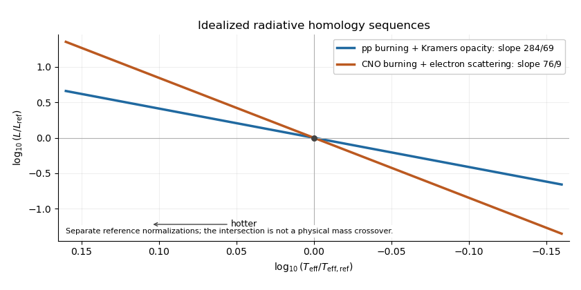
Logarithmic Hertzsprung-Russell slopes for the two idealized radiative homology sequences, with temperature increasing to the left
. Details. The proton–proton/Kramers model applies to the lower-mass regime; the CNO/electron-scattering model applies to the higher-mass regime. Higher-mass cores are hotter, making the more temperature-sensitive CNO cycle efficient, and highly ionized material favors electron-scattering opacity. These are the stated idealized radiative, gas-pressure-supported sequences: a fully convective low-mass star or a radiation-pressure-dominated massive star needs a different structural model. The intersection of independently normalized lines in the figure does not specify a physical crossover mass.
Past exam of the mathematics course of the University of Cambridge 2016 iii Paper 317 2 b Solution by Codex 0 Created 2026-10-03 Updated 2026-10-14
Codex 0 Created 2026-10-03 Updated 2026-10-14For PP chain burning and the Kramers' opacity law, insert , , and into the homology relations for radiative stars:Thus the radiative homology with proton-proton burning and Kramers opacity isTo obtain the Hertzsprung-Russell diagram slope, apply the Stefan–Boltzmann law :Equivalently . The Hertzsprung-Russell slope of a stellar homology sequence refers here to logarithmic luminosity versus logarithmic effective temperature; a conventional diagram reverses its horizontal axis, so the line descends toward the right.
Past exam of the mathematics course of the University of Cambridge 2016 iii Paper 317 2 a Solution by Codex 0 Created 2026-10-03 Updated 2026-10-06
Codex 0 Created 2026-10-03 Updated 2026-10-06Use stellar homology: dimensionless profiles and composition are fixed, so proportionality constants do not change along the model sequence. Scaling mass conservation and the stellar hydrostatic equation giveswhere the last relation uses the ideal gas equation of state with fixed mean molecular weight. The specific stellar energy-generation rate is , soBy stellar radiative diffusion, , henceEquate the generated and transported luminosity in thermal equilibrium. The homology relations for radiative stars giveThis division presumes a nonzero denominator. If it vanishes, the scaling balance instead imposes a condition on or leaves the radius scaling undetermined, depending on the numerator. For later use, the corresponding mass-luminosity relation exponent is
Past exam of the mathematics course of the University of Cambridge 2016 iii Paper 317 1 d Solution by Codex 0 Created 2026-10-03 Updated 2026-10-06
Codex 0 Created 2026-10-03 Updated 2026-10-06Compare two cooling states of the same white dwarf, holding its mass, nearly temperature-independent degenerate radius and composition fixed. The matching of a white-dwarf envelope to a degenerate core gives , while the geometrical thickness of a white-dwarf radiative envelope gives at leading thin-layer order. Eliminate :Thus a luminosity drop makes the envelope thinner, with . This is the white-dwarf envelope thickness-luminosity relation. Retaining finite thickness in the radiative-zero model gives the correctionwhich reduces to the boxed result for .
Past exam of the mathematics course of the University of Cambridge 2016 iii Paper 317 1 c Solution by Codex 0 Created 2026-10-03 Updated 2026-10-06
Codex 0 Created 2026-10-03 Updated 2026-10-06Apply the preceding temperature profile at the envelope base. Introduce the dimensionless parameterThen , so the geometrical thickness of a white-dwarf radiative envelope isThe smallness to be established is therefore , up to the numerical factor .
That ordering follows from the cold, strongly electron-degenerate white dwarf model. Throughout the mass-bearing core, , where is the Fermi energy. For nonrelativistic electron degeneracy pressure,The stellar hydrostatic equation gives a characteristic core of order . Consequentlyfor fixed composition with order-one molecular-weight ratios, and . Equivalently, the matched base mass density is much lower than a characteristic core mass density, since . The degeneracy ordering applies in the bulk core; at the matching point degeneracy is becoming marginal.
The inequalities and express different facts. The first justifies ignoring surface-temperature terms, while the second makes the envelope geometrically thin. If the core were hot enough that were not small, the exact expression would not justify a thin-layer approximation.
Past exam of the mathematics course of the University of Cambridge 2016 iii Paper 317 1 b Solution by Codex 0 Created 2026-10-03 Updated 2026-10-06
Codex 0 Created 2026-10-03 Updated 2026-10-06In the radiative-zero white-dwarf envelope, . Substitute this derivative into the stellar hydrostatic equation:Integrating from the idealized zero-temperature surface at givesThis also gives . A finite surface temperature adds to the integrated profile if the pure power-law pressure relation is retained locally. Near the actual photosphere, the integration constant in the pressure law also matters; the displayed expression is the radiative-zero limit implicit in the printed result and accurate in the deep envelope when .
Past exam of the mathematics course of the University of Cambridge 2016 iii Paper 317 1 a Solution by Codex 0 Created 2026-10-03 Updated 2026-10-14
Codex 0 Created 2026-10-03 Updated 2026-10-14Write for the specific gas constant, with the printed denoting the atomic mass unit, and for the radiation constant. In the low-mass envelope the enclosed mass is approximately and the outward luminosity is approximately . The stellar hydrostatic equation, stellar radiative diffusion, and ideal gas equation giveThe Kramers' opacity law becomes . Dividing the two differential equations eliminates radius and mass density:Integrating from a surface matching point givesDeep compared with the photosphere, the surface terms are negligible. The radiative-zero white-dwarf envelope therefore hasThis is the leading envelope approximation used in the later parts, rather than an exact atmospheric boundary condition at .
At the base, temperature, mass density and pressure match the isothermal degenerate core. Let , where is the mean molecular weight per electron. Equating the gas and electron degeneracy pressure givesHence . Substituting this into the envelope relation at yieldsThe matching of a white-dwarf envelope to a degenerate core thus gives , the envelope relation underlying Mestel's cooling law. It depends on pressure as well as mass density continuity at the interface; otherwise the supplied core equation would not determine the matching mass density.
Past exam of the mathematics course of the University of Cambridge 2016 iii Paper 315 4 j Solution by Codex 0 Created 2026-10-03 Updated 2026-10-31
Codex 0 Created 2026-10-03 Updated 2026-10-31Three solar-system effects illustrate chemical disequilibrium. First, vertical mixing carries carbon monoxide from hot deep regions into cooler observable layers of giant planets, where its local-equilibrium abundance would be small. Second, phosphine survives in the observable atmospheres of Jupiter and Saturn because deep supply competes with its destruction, making it a tracer of transport. Third, methane photolysis creates hydrocarbons such as ethane and acetylene, and can help form upper-atmospheric atmospheric hazes in giant planets and Titan.
Three exoplanet effects are complementary. First, carbon monoxide–methane quenching can keep carbon monoxide abundant and methane depleted in cool observable gas, including hot-Neptune/giant atmospheres that would locally favor methane. Second, atmospheric photochemistry dissociates methane/Ammonia and produces radicals, hydrogen cyanide, hydrocarbons and possibly atmospheric hazes, changing spectral bands from their equilibrium strengths. Third, horizontal chemical quenching can preserve hot-dayside carbon chemistry on the cooler nightside/terminator and reduce the abundance contrast expected from separate local-equilibrium columns.
Transport, photon-driven reactions and finite chemical adjustment times change the observable composition. The effects are conditional on the species' chemical timescale relative to mixing, advection and irradiation; they do not imply that every molecule is out of equilibrium everywhere.
Pinned article: Introduction to the OurBigBook Project
Welcome to the OurBigBook Project! Our goal is to create the perfect publishing platform for STEM subjects, and get university-level students to write the best free STEM tutorials ever.
Everyone is welcome to create an account and play with the site: ourbigbook.com/go/register. We belive that students themselves can write amazing tutorials, but teachers are welcome too. You can write about anything you want, it doesn't have to be STEM or even educational. Silly test content is very welcome and you won't be penalized in any way. Just keep it legal!
Intro to OurBigBook
. Source. We have two killer features:
- topics: topics group articles by different users with the same title, e.g. here is the topic for the "Fundamental Theorem of Calculus" ourbigbook.com/go/topic/fundamental-theorem-of-calculusArticles of different users are sorted by upvote within each article page. This feature is a bit like:
- a Wikipedia where each user can have their own version of each article
- a Q&A website like Stack Overflow, where multiple people can give their views on a given topic, and the best ones are sorted by upvote. Except you don't need to wait for someone to ask first, and any topic goes, no matter how narrow or broad
This feature makes it possible for readers to find better explanations of any topic created by other writers. And it allows writers to create an explanation in a place that readers might actually find it.
Figure 1. Screenshot of the "Derivative" topic page. View it live at: ourbigbook.com/go/topic/derivativeVideo 2. OurBigBook Web topics demo. Source. - local editing: you can store all your personal knowledge base content locally in a plaintext markup format that can be edited locally and published either:This way you can be sure that even if OurBigBook.com were to go down one day (which we have no plans to do as it is quite cheap to host!), your content will still be perfectly readable as a static site.
- to OurBigBook.com to get awesome multi-user features like topics and likes
- as HTML files to a static website, which you can host yourself for free on many external providers like GitHub Pages, and remain in full control

Figure 2. You can publish local OurBigBook lightweight markup files to either OurBigBook.com or as a static website.
Figure 3. Visual Studio Code extension installation.
Figure 5. . You can also edit articles on the Web editor without installing anything locally. Video 3. Edit locally and publish demo. Source. This shows editing OurBigBook Markup and publishing it using the Visual Studio Code extension. 
- Infinitely deep tables of contents:




All our software is open source and hosted at: github.com/ourbigbook/ourbigbook
Further documentation can be found at: docs.ourbigbook.com
Feel free to reach our to us for any help or suggestions: docs.ourbigbook.com/#contact